Street Journal domain show a reduction in average word error rate of over 20%. This paper concludes with a discussion of intrinsic tradeoffs, such as the ...
Exploiting Latent Semantic Information in Statistical Language Modeling JEROME R. BELLEGARDA, SENIOR MEMBER, IEEE Invited Paper
Statistical language models used in large-vocabulary speech recognition must properly encapsulate the various constraints, both local and global, present in the language. While local constraints are readily captured through n-gram modeling, global constraints, such as long-term semantic dependencies, have been more difficult to handle within a data-driven formalism. This paper focuses on the use of latent semantic analysis, a paradigm that automatically uncovers the salient semantic relationships between words and documents in a given corpus. In this approach, (discrete) words and documents are mapped onto a (continuous) semantic vector space, in which familiar clustering techniques can be applied. This leads to the specification of a powerful framework for automatic semantic classification, as well as the derivation of several language model families with various smoothing properties. Because of their large-span nature, these language models are well suited to complement conventional n-grams. An integrative formulation is proposed for harnessing this synergy, in which the latent semantic information is used to adjust the standard n-gram probability. Such hybrid language modeling compares favorably with the corresponding n-gram baseline: experiments conducted on the Wall Street Journal domain show a reduction in average word error rate of over 20%. This paper concludes with a discussion of intrinsic tradeoffs, such as the influence of training data selection on the resulting performance. Keywords—Latent semantic analysis, multispan integration,
n-grams, speech recognition, statistical language modeling. I. INTRODUCTION
Language modeling plays a pivotal role in automatic speech recognition (ASR). It is variously used to constrain the acoustic analysis, guide the search through various (partial) text hypotheses, and/or contribute to the determination of the final transcription [1], [40], [57]. Fundamentally, its function is to encapsulate as much as possible of the syntactic, semantic, and pragmatic characteristics for the task considered. The successful capture of this information is critical to help determine the most likely sequence of words spoken because it quantifies which word sequences Manuscript received December 23, 1999; revised April 12, 2000. The author is with the Spoken Language Group, Apple Computer, Inc., Cupertino, CA 95014 USA. Publisher Item Identifier S 0018-9219(00)08093-2.
are acceptable in a given language for a given task and which are not. Thus, language modeling can be thought of as a way to impose a collection of constraints on word sequences. In the two past decades, statistical -grams have steadily emerged as the preferred way to impose such constraints in a wide range of domains [21]. The reader is referred to [61] and [72] for a comprehensive overview of the state-of-the-art in the field, including an insightful perspective on -grams in light of other techniques, and an excellent tutorial on challenges lying ahead. Some of these challenges are further considered below. A. Locality Problem The success of an -gram in capturing relevant syntactic, semantic, and pragmatic information from the training data is directly related to its ability to suitably discriminate between different strings of words. This ability is heavily influenced by two related issues, coverage and estimation. Coverage hinges on the selection of the underlying vocabulary, with tradeoffs such as incurring more errors due to unknown words (low coverage) versus losing accuracy from increased acoustic confusability (very large vocabulary) [59]. This paper is more concerned with the estimation issue, which centers around the choice of . There, the major tradeoff has to do with settling for weaker predictive power (low ) versus suffering from more unreliable parameter estimates (higher ) [53]. In practice, parameter reliability demand low values of (see, e.g., [45] and [54]), which in turn imposes an artificially local horizon to the language model. As a result, -grams as typically derived are inherently unable to capture large-span relationships in the language. Consider, for instance, predicting the word “fell” from the word “stocks” in the two equivalent phrases: stocks fell sharply as a result of the announcement
and
(1)
stocks, as a result of the announcement, sharply fell
(2)
0018–9219/00$10.00 © 2000 IEEE
PROCEEDINGS OF THE IEEE, VOL. 88, NO. 8, AUGUST 2000
1279
In (1), the prediction can be done with the help of a bigram ). This is straightforward with the language model ( kind of resources currently available [58]. In (2), however, would be necessary, a rather unrealistic the value proposition at the present time. In large part because of this inability to reliably capture large-span behavior, the performance of conventional -gram technology has essentially reached a plateau [61], [72]. This observation has sparked interest in a variety of research directions, mostly relying on either information aggregation or span extension [11]. Information aggregation increases the reliability of the parameter estimation by taking advantage of exemplars of other words that behave “like” this word in the particular context considered. The tradeoff, typically, is higher robustness at the expense of a loss in resolution. This paper is more closely aligned with span extension, which extends and/or complements the -gram paradigm with information extracted from large-span units (i.e., comprising a large number of words). The tradeoff here is in the choice of units considered, which has a direct effect on the type of long-distance dependencies modeled. These units tend to be either syntactic or semantic in nature. We now expand on these two choices.
B. Syntactically Driven Span Extension Assuming a suitable parser is available for the domain considered, syntactic information can be used to incorporate large-span constraints into the recognition. How these constraints are incorporated varies from estimating -gram probabilities from grammar-generated data [70] to computing a linear interpolation of the two models [43]. Most recently, syntactic information has been used specifically to determine equivalence classes on the -gram history, resulting in so-called dependency language models [19], [56], sometimes also referred to as structured language models [20], [42], [66]. In that framework, each unit is in the form of the headword of the phrase spanned by the associated parse subtree. The standard -gram language model is then modified to operate headwords as opposed to the last given the last words. Said another way, the structure of the model is no longer predetermined: which words serve as predictors depends on the dependency graph, which is a hidden variable [61], [72]. In the example above, the top two headwords in the dependency graph would be “stocks” and “fell” in both cases, thereby solving the problem. The main caveat in such modeling is the reliance on the parser, and particularly the implicit assumption that the correct parse will in fact be assigned a high probability [69]. The basic framework was recently extended to operate efficiently in a left-to-right manner [20], [42], through careful optimization of both chart parsing [67] and search modules. Also noteworthy is a somewhat complementary line of research [68], which exploits the syntactic structure contained in the sentences prior to the one featuring the word being predicted. 1280
C. Semantically Driven Span Extension High-level semantic information can also be used to incorporate large-span constraints into the recognition. Since by nature such information is diffused across the entire text being created, this requires the definition of a document as a semantically homogeneous set of sentences. Then each document can be characterized by drawing from a (possibly large) set of topics, usually predefined from a hand-labeled hierarchy, which covers the relevant semantic domain [39], [63], [64]. The main uncertainty in this approach is the granularity required in the topic clustering procedure [31]. To illustrate, in (1) and (2), even perfect knowledge of the general topic (most likely, “stock market trends”) does not help much. An alternative solution is to use long distance dependencies between word pairs which show significant correlation in the training corpus. In the above example, suppose that the training data reveals a significant correlation between “stocks” and “fell.” Then the presence of “stocks” in the document could automatically trigger “fell,” causing its probability estimate to change. Because this behavior would occur in both (1) and in (2), proximity being irrelevant in this kind of model, the two phrases would lead to the same result. In this approach, the pair (stocks, fell) is said to form a word trigger pair [51]. In practice, word pairs with high mutual information are searched for inside a window of fixed duration. Unfortunately, trigger pair selection is a complex issue: different pairs display markedly different behavior, which limits the potential of low-frequency word triggers [60]. Still, self-triggers have been shown to be particularly powerful and robust [51], which underscores the desirability of exploiting correlations between the current word and features of the document history. Recent work has sought to extend the word trigger concept by using a more comprehensive framework to handle the trigger pair selection [3]–[10], [12], [24], [34], [36]. This is based on a paradigm originally formulated in the context of information retrieval, called latent semantic analysis (LSA) [15], [27], [30], [32], [37], [49], [50], [65]. In this paradigm, co-occurrence analysis still takes place across the span of an entire document, but every combination of words from the vocabulary is viewed as a potential trigger combination. This leads to the systematic integration of long-term semantic dependencies into the analysis. The concept of document assumes that the available training data is tagged at the document level, i.e., there is a way to identify article boundaries. This is the case, for example, with the ARPA North American Business (NAB) News corpus [46]. Once this is done, the LSA paradigm can be used for word and document clustering [12], [34], [36], as well as for language modeling [3], [6], [24]. In all cases, it was found to be suitable to capture some of the global semantic constraints present in the language. In fact, hybrid -gram LSA language models, constructed by embedding LSA into the standard -gram formulation, were shown to result in a substantial reduction in both perplexity [5], [6] and average word error rate [7]–[10]. PROCEEDINGS OF THE IEEE, VOL. 88, NO. 8, AUGUST 2000
D. Organization The focus of this paper is on semantically driven span extension only, and more specifically on how the LSA paradigm can be exploited to improve statistical language modeling. The main objectives are: 1) to review the data-driven extraction of latent semantic information; 2) to assess its potential use in the context of spoken language processing; 3) to describe its integration with conventional -gram language modeling; 4) to examine the behavior of the resulting hybrid models in speech recognition experiments; 5) to discuss a number of factors that influence performance. This paper is organized as follows. In the next two sections, we give an overview of the mechanics of LSA feature extraction, as well as the salient characteristics of the resulting LSA feature space. Section IV explores the applicability of this framework for general semantic classification. In Section V, we shift the focus to LSA-based statistical language modeling for large-vocabulary recognition. Section VI describes the various smoothing possibilities available to make LSA-based language models more robust. In Section VII, we illustrate some of the benefits associated with hybrid -gram LSA modeling on a subset of the Wall Street Journal (WSJ) task. Finally, Section VIII discusses the inherent tradeoffs associated with the approach, as evidenced by the influence of the data selected to train the LSA component of the model. II. LATENT SEMANTIC ANALYSIS Let , , be some underlying vocabulary and a training text corpus, comprising articles (documents) relevant to some domain of interest (like business news, e.g., and in the case of the NAB corpus [46]). Typically, may be on the order of 10 000 and 100 000, respectively; might comprise a hundred million words or so. The LSA paradigm defines a mapping between the discrete sets , and in is a continuous vector space , whereby each word represented by a vector in , and each document in is represented by a vector in . A. Feature Extraction The starting point is the construction of a matrix ( ) of co-occurrences between words and documents. In marked contrast with -gram modeling, word order is ignored, which is of course in line with the semantic nature of the approach [50]. This makes it an instance of the so-called “bag-of-words” paradigm, which disregards collocational information in word strings: the context for each word essentially becomes the entire document in which it appears. is accumulated from the available Thus, the matrix training data by simply keeping track of which word is found in what document. This accumulation involves some suitable function of the word count, i.e., the number of times each word appears in BELLEGARDA: STATISTICAL LANGUAGE MODELING
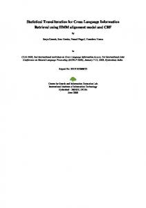
each document [12]. Various implementations have been investigated by the information retrieval community (see, e.g., [29]). Evidence points to the desirability of normalizing for document length and word entropy. Thus, a suitable expression for the cell of is (3) where number of times occurs in ; total number of words present in ; normalized entropy of in the corpus . reflects the fact that The global weighting implied by two words appearing with the same count in do not necessarily convey the same amount of information about the document; this is subordinated to the distribution of the words in the collection . the total number of times If we denote by occurs in , the expression for is easily seen to be (4) , with equality if and only if By definition, and , respectively. A value of close to 1 indicates a word distributed across many documents throughout the corpus, while a value of close to 0 means that the word is present only in a few specific docuis, therefore, a measure of ments. The global weight the indexing power of the word . B. Singular Value Decomposition ) word-document matrix resulting from The ( the above feature extraction defines two vector representacan be tions for the words and the documents. Each word uniquely associated with a row vector of dimension , and each document can be uniquely associated with a column vector of dimension . Unfortunately, these vector representations are unpractical for three related reasons. First, the and can be extremely large; second, the dimensions and are typically very sparse; and third, the vectors two spaces are distinct from one other. To address these issues, it is useful to employ singular value decomposition (SVD), a technique closely related to eigenvector decomposition and factor analysis [35]. We proas follows: ceed to perform the (order- ) SVD of (5) where ( ) left singular matrix with ); row vectors ( ( ) diagonal matrix of singular ; values ( ) right singular matrix with ); row vectors ( order of the decomposition; matrix transposition. 1281
Fig. 1. Singular value decomposition (after [44]).
As is well known, both left and right singular matrices and are column-orthonormal, i.e., (the identity matrix of order ). Thus, the column vectors of and each define an orthonormal basis for the space spanned by the ( -dimensional) ’s and of dimension ’s. Furthermore, it can be shown (see [25]) that the matrix is the best rank- approximation to the word-document matrix , for any unitarily invariant norm. This entails, for any matrix of rank (6) refers to the norm and is the smallest where SVD of . Obsingular value retained in the orderif is equal to the rank of . viously, Following [44], this decomposition can be illustrated as (i.e., words) are projected in Fig. 1. The row vectors of onto the orthonormal basis formed by the column vectors of the right singular matrix , or, equivalently, the row vec(top figure). This defines a new representation tors of for the words, in terms of their coordinates in this projection, 1282
namely, the rows of . In essence, the row vector characterizes the position of word in the underlying -dimen. Similarly, the column vectors sional space, for (i.e., documents) are projected onto the orthonormal of basis formed by the column vectors of the left singular matrix (middle figure). The coordinates of the documents in . This this space are, therefore, given by the columns of , or, equivalently, in turn means that the column vector , characterizes the position of document the row vector in dimensions, for . We refer to each of scaled vectors as a word vector, uniquely the in the vocabulary, and each of the associated with word scaled vectors as a document vector, uniquely associated with document in the corpus (bottom figure). C. Interpretation This amounts to representing each word and each document as a linear combination of (hidden) abstract concepts, which arise automatically from the SVD mechanism [44]. Since the SVD provides, by definition, a parsimonious description of the linear space spanned by , we can infer that PROCEEDINGS OF THE IEEE, VOL. 88, NO. 8, AUGUST 2000
this set of abstract concepts is specified to minimally span the words in the vocabulary and the documents in the corpus . Thus, the dual one-to-one mapping embodied in (5), between words/documents and word/document vectors, corresponds to an efficient representation of the training data. Essentially, (5) defines a transformation between high-dimensional discrete entities ( and ) and a low-dimensional continuous vector space , the -dimensional space spanned by the ’s and ’s. The dimension is bounded from above by and from below by the the (unknown) rank of the matrix amount of distortion tolerable in the decomposition. Values to are typically used of in the range for information retrieval [30]. In the present context, we have to work reasonably well. found captures the major The basic idea behind (5) is that structural associations in and ignores higher order effects. The “closeness” of vectors in the LSA space is, therefore, determined by the overall pattern of the language used in , as opposed to specific constructs. Hence, two words whose representations are “close” (in some suitable metric) tend to appear in the same kind of documents, whether or not they actually occur within identical word contexts in those documents. Conversely, two documents whose representations are “close” tend to convey the same semantic meaning, whether or not they contain the same word constructs. Thus, we can expect that the respective representations of words and documents that are semantically linked would also be “close” in the LSA space . Of course, the optimality of this framework can be denorm arising from (6) is probbated, since the underlying ably not the best choice when it comes to linguistic phenomena. Depending on many subtly intertwined factors like frequency and recency, linguistic co-occurrences may not always have the same interpretation. When comparing word counts, for example, observing 100 occurrences versus 99 is markedly different from observing one versus zero. This has motivated the investigation of an alternative objective function based on the Kullback–Leibler divergence [37]. This approach has the advantage of providing an elegant probabilistic interpretation of (5), at the expense of requiring a conditional independence assumption on the words and the documents [38]. This can be viewed as an instance of the familiar tradeoff between tractability and modeling accuracy. This caveat notwithstanding, the correspondence between closeness in LSA space and semantic relatedness is well documented. In applications such as information retrieval, filtering, induction, and visualization, the LSA framework has repeatedly proven remarkably effective in capturing semantic information [15], [27], [30], [32], [38], [49], [50], [65]. An illustration of this fundamental behavior was recently provided in [55], [71], in the context of an (artificial) information retrieval task with 20 distinct topics and a vocabulary of 2000 words. A probabilistic corpus model generated 1000 documents, each 50 to 100 words long. The probability distribution for each topic was such that 0.95 of its probability density was equally distributed among topic words, and the BELLEGARDA: STATISTICAL LANGUAGE MODELING
Fig. 2. Improved topic separability in LSA space (after [55], [71]).
remaining 0.05 was equally distributed among all the 2000 words in the vocabulary. The authors of the study measured the distance between all pairs of documents, both in the original space and in the LSA space obtained as above, with . This leads to the expected distance distributions depicted in Fig. 2, where a pair of documents is considered “intratopic” if the two documents were generated from the same topic and “intertopic” otherwise. It can be seen that in the LSA space, the average distance between intertopic pairs stays about the same, while the average distance between intratopic pairs is dramatically reduced. In addition, the standard deviation of the intratopic distance distribution also becomes substantially smaller. As a result, separability between intra- and intertopic pairs is much better in the LSA space than in the original space. Note that this holds in spite of a sharp increase in the standard deviation of the intertopic distance distribution, which bodes well for the general applicability of the method. Analogous observations can be made regarding the distance between words and/or between words and documents. D. (Off-Line) Computational Effort Clearly, classical methods for determining the SVD of dense matrices (see, e.g., [16]) are not optimal for . Because these methods large sparse matrices such as apply orthogonal transformations (Householder or Givens) directly to the input matrix, they incur excessive fill-in and thereby require tremendous amounts of memory. In ; but addition, they compute all the singular values of , and, therefore, doing so is compuhere tationally wasteful. Instead, it is more appropriate to solve a sparse symmetric eigenvalue problem, which can then be used to indirectly compute the sparse singular value decomposition. Several suitable iterative algorithms have been proposed by Berry, based on either the subspace iteration or the Lanczos recursion method [14]. The primary cost of these algorithms lies in the total number of sparse matrix-vector multiplications rethe density of , defined as the quired. Let us denote by divided by the product total number of nonzero entries in 1283
of its dimensions . Then the total cost in floating-point operations per iteration is given by [14]
between words is, therefore, the cosine of the angle between and . Thus
(7) hovers in the range 0.25% to 0.5% In a typical case, (see [30]), and the value of is between 100 to 200. This expression can, therefore, be approximated by (8) and mentioned earlier, this correFor the values of sponds to a few billion floating-point operations (flops) per iteration. On any midrange desktop machine (such as a 400-MHz Apple iMac DV, rated at approximately 60 Mflops), this translates into (up to) a few minutes of CPU time. As convergence is typically achieved after 100 or so iterations, the entire decomposition is usually completed within a matter of hours. III. LSA FEATURE SPACE In the continuous vector space obtained above, each is represented by the associated word vector word , and each document is of dimension , represented by the associated document vector of dimension , . This opens up the opportunity to apply familiar clustering techniques in , as long as a distance measure consistent with the SVD formalism is defined on the vector space. The nice thing about this form of clustering is that it takes the global context into account, as opposed to conventional -gram-based clustering methods, which only consider collocational effects. embodies, by construction, all strucSince the matrix tural associations between words and documents, it follows characterizes all that, for a given training corpus, characterizes co-occurrences between words, and all co-occurrences between documents. Thus, the extent to and have a similar pattern of occurrence which words across the entire set of documents can be inferred from the cell of , and the extent to which documents and contain a similar pattern of words from the entire cell of . vocabulary can be inferred from the A. Word Clustering Expanding obtain1
using the SVD expression (5), we
(9) cell of Since is diagonal, this means that the can be obtained by taking the dot product between the th , namely, and . We and th rows of the matrix conclude that a natural metric to consider for the “closeness” 1Henceforth, we ignore the distinction between W and W ^ . From (6), this is without loss of generality under the assumption that R is chosen to be equal to the rank of W .
1284
(10) . A value of means for any the two words always occur in the same semantic context, means the two words are while a value of used in increasingly different semantic contexts. While (10) does not define a bona fide distance measure in the space , , it easily leads to one. For example, over the interval the measure (11) can be readily verified to satisfy the properties of a distance on . Once (11) is specified, it is straightforward to proceed with the clustering of the word vectors , using any of a variety of algorithms (see, for instance, [2]). Since the number of such vectors is relatively large, it is advisable to perform this clustering in stages, using, for example, K-means and bottom-up clustering sequentially. In that case, K-means clustering is used to obtain a coarse partition of the vocabulary in to a small set of superclusters. Each supercluster is then itself partitioned using bottom-up clustering, resulting in a final set . This process can be thought of of clusters , as uncovering, in a data-driven fashion, a particular layer of semantic knowledge in the space . B. Word Cluster Example For the purpose of illustration, we recall here the result of a word clustering experiment originally reported in [6]. documents was randomly selected A corpus of from the WSJ portion of the NAB corpus. LSA training was then performed with an underlying vocabulary of words, and the word vectors in the resulting LSA space were clustered into 500 disjoint clusters as explained above. Two representative examples of the clusters so obtained are shown in Fig. 3. The first thing to note is that these word clusters comprise words with different part of speech, a marked difference with conventional class -gram techniques (see [53]). This is a direct consequence of the semantic nature of the derivation. Second, some obvious words seem to be missing from the clusters: e.g., the singular noun “drawing” from cluster 1 and the present tense verb “rule” from cluster 2. This is an instance of a phenomenon called polysemy: “drawing” and “rule” are more likely to appear in the training text with their alternative meanings (as in “drawing a conclusion” and “breaking a rule,” respectively), thus resulting in different cluster assignments. Finally, some words seem to contribute only marginally to the clusters: e.g., “hysteria” from cluster 1 and “here” from cluster 2. These are the unavoidable outliers at the periphery of the clusters. PROCEEDINGS OF THE IEEE, VOL. 88, NO. 8, AUGUST 2000
Fig. 3. Word cluster example (after [6]).
C. Document Clustering using the SVD
Proceeding as above, expanding expression (5) yields
(12) cell of can be obAgain, this means that the tained by taking the dot product between the th and th , namely, and . As a recolumns of the matrix sult, a natural metric to consider for the “closeness” between documents is the cosine of the angle between and . Thus (13) . This has the same functional form for any as (10), and, therefore, the distance (11) is equally valid for both word and document clustering.2 Earlier comments regarding clustering implementation , apply here as well. The end result is a set of clusters , which can be viewed as representing another layer of semantic knowledge in the space . D. Document Cluster Example An early document clustering experiment using the above measure was documented in [36]. This work was conducted on the British National Corpus (BNC), a heterogeneous corpus that contains a variety of hand-labeled topics. Using the LSA framework as above, it is possible to partition BNC into distinct clusters and compare the subdomains so obtained with the hand-labeled topics provided with the corpus. This comparison was conducted by evaluating two different mixture trigram language models: one built using the LSA subdomains and one built using the hand-labeled topics. As the perplexities obtained were very similar [36], this validates the automatic partitioning performed using LSA. Some evidence of this behavior is provided in Fig. 4, which plots the distributions of four of the hand-labeled 2In fact, the measure (11) is precisely the one used in the study reported in Fig. 2. Thus, the distances on the x axis of Fig. 2 are (d ; d ) expressed in radians.
D
BELLEGARDA: STATISTICAL LANGUAGE MODELING
Fig. 4. Document cluster example (after [36]).
BNC topics against the ten-document subdomains automatically derived using LSA. While clearly not matching the hand-labeling, LSA document clustering in this example still seems reasonable. In particular, as one would expect, the distribution for the natural science topic is relatively close to the distribution for the applied science topic (see the two solid lines), but quite different from the two other topic distributions (in dashed lines). From that standpoint, the data-driven LSA clusters appear to adequately cover the semantic space. IV. SEMANTIC CLASSIFICATION As seen in the previous two sections, the latent semantic framework has a number of interesting properties, including: 1) a single-vector representation for both words and documents in the same continuous vector space; 2) an underlying topological structure reflecting semantic similarity; 3) a well-motivated, natural metric to measure the distance between words and between documents in that space; 4) a relatively low dimensionality, which makes clustering meaningful and practical. These properties can be exploited in several areas of spoken language processing. In this section, we address the most 1285
immediate domain of application, which follows directly from the previous clustering discussion: (data-driven) semantic classification [4], [18], [22], [33]. A. Framework Extension Semantic classification refers to the task of determining, for a given document, which one of several predefined topics the document is most closely aligned with. In contrast with the clustering setup discussed above, such a document will not (normally) have been seen in the training corpus. Hence, we first need to extend the LSA framework accordingly. As it turns out, under relatively mild assumptions, finding a representation for a new document in the space is straightforward. , where Let us denote the new document by , with the tilde symbol reflects the fact that the document was not part of the training data. First, we construct a feature vector containing, for each word in the underlying vocabulary, the . This feature vector , a weighted counts (3) with column vector of dimension , can be thought of as an additional column of the matrix . Thus, provided the matrices and do not change, the SVD expansion (5) implies (14) act as an additional where the -dimensional vector . This in turn leads to the definition column of the matrix (15) The vector , indeed seen to be functionally similar to a document vector, corresponds to the representation of the new document in the space . This is illustrated in Fig. 5, rendition of , with x’s and o’s dewhich depicts the noting the original words and documents, respectively, and the symbol “@” showing the location of the new document. To convey the fact that it was not part of the SVD extracis referred to as a pseudodocution, the new document ment. Recall that the set of abstract concepts arising from the SVD mechanism is specified to minimally span and . As a result, if the new document contains language patterns that are inconsistent with those extracted from , the SVD expansion (5) will no longer apply. Similarly, if the addition of causes the major structural associations in to shift in some substantial manner, the set of abstract concepts will become inadequate. Then and will no longer be valid, in which case it would be necessary to recompute (5) to find a proper representation for . If, on the other hand, the new document generally conforms to the rest of the corpus , then the pseudodocument vector in (15) will be a reasonable representation for . Once the representation (15) is obtained, the “closeness” and any document cluster between the new document (i.e., words) are projected onto Fig. 1. The row vectors of can then be expressed as , calculated from the (13) in the previous section. 1286
Fig. 5.
Latent semantic vector space S (R = 2).
B. Semantic Inference This can be readily exploited in command-and-control tasks, such as desktop command-and-control [4] or automated call routing [18]. Suppose that each document cluster can be uniquely associated with a particular action in the task. Then the centroid of each cluster can be viewed as the semantic representation of this action in the LSA space. Said another way, each centroid becomes a semantic anchor for the corresponding action. A particularity of these semantic anchors is that they are automatically derived from the evidence presented during training, without regard to the particular syntax used to express the semantic link between various word sequences and the corresponding action. This opens up the possibility of mapping an unknown word sequence (treated as a new “document”) onto an action by computing the distance (11) between that “document” and each semantic anchor and picking the minimum. In principle, this approach, which we refer to as semantic inference [4], allows for any word constructs in the formulation of the command/query. It is, therefore, best used in conjunction with a speech-recognition system using a statistical language model. (A typical implementation framework is illustrated in Fig. 6.) In contrast with usual inference engines (see [26]), semantic inference thus defined does not rely on formal behavioral principles extracted from a knowledge base. Instead, the domain knowledge is automatically encapsulated in the LSA space in a data-driven fashion. As a result, semantic inference replaces the traditional rule-based mapping between utterance and action by a data-driven classification, which can be thought of as a way to perform “bottom-up” natural language understanding [52]. This makes it possible to relax some of the typical command-and-control interaction constraints. For example, it obviates the need to specify rigid language constructs through a domain-specific (and, thus, typically hand-crafted) finite-state grammar. This is turn allows the end user more flexibility in expressing the desired command/query, which tends to reduce the associated cognitive load and thereby enhance user satisfaction [18]. C. Caveats Recall that LSA is an instance of the “bag-of-words” paradigm, which pays no attention to the order of words in the sentence. This is what makes it well suited to capture semantic relationships between words. By the same token, however, it is inherently unable to capitalize on the local PROCEEDINGS OF THE IEEE, VOL. 88, NO. 8, AUGUST 2000
A. LSA Component Let denote the word about to be predicted and the admissible LSA history (context) for this particular word. At best this history can only be the current document so far, i.e., , which we denote by . Thus, in general up to word terms, the LSA language model probability is given by (18)
Fig. 6.
Semantic inference for command and control.
(syntactic, pragmatic) constraints present in the language. For tasks such as call routing, where the broad topic of a message is to be identified, this limitation is probably inconsequential. For general command and control tasks, however, it may be a great deal more severe. Imagine two commands that differ only in the presence of the word “not” in a crucial place. The respective vector representations could conceivably be relatively close in the LSA space but would obviously have vastly different intended consequences. Worse yet, some commands may differ only through word order. Consider, for instance, the two actual MacOS 9 commands change pop-up to window
(16)
change window to pop-up
(17)
and
These two commands are mapped onto the exact same point in LSA space, which makes them utterly impossible to disambiguate. As it turns out, it is possible to handle such cases through an extension of the basic LSA framework using word agglomeration. The idea is to move from the characterization of co-occurrences between words and documents to the characterization of co-occurrences between word -tuples and documents, where each word -tuple is the agglomeration of successive words and each original document is now expressed in terms of all the word -tuples it contains. Despite the resulting increase in computational complexity, this extension is practical in the context of semantic classification because of the relatively modest dimensions involved (as compared to large vocabulary recognition). More details would be beyond the scope of this manuscript, but the reader is referred to [13] for further discussion. V.
-GRAM
LSA LANGUAGE MODELING
Another major area of application of the LSA framework is in statistical language modeling, where it can readily serve as a paradigm for semantically driven span extension. Because of the limitation just discussed, however, it is best applied in conjunction with the standard -gram approach. This section describes how this can be done. BELLEGARDA: STATISTICAL LANGUAGE MODELING
where the conditioning on reflects the fact that the probability depends on the particular vector space arising from is the SVD representation. In this expression, computed directly from the representations of and in the space , i.e., it is inferred from the “closeness” between the associated word vector and (pseudo)document vector in . We, therefore, have to specify both the appropriate pseudodocument representation and the relevant probability measure. 1) Pseudodocument Representation: To come up with a pseudodocument representation, we leverage the results of Section IV-A, with some slight modifications due to the time-varying nature of the span considered. From (15), the has a representation in the space given by context (19) is As mentioned before, this vector representation for adequate under some consistency conditions on the general patterns present in the domain considered. The difference with Section IV-A is that, as increases, the content of the new document grows, and, therefore, the pseudodocument vector moves around accordingly in the LSA space. Assuming the new document is semantically homegeneous, eventually we can expect the resulting trajectory to settle down in the vicinity of the document cluster corresponding to the closest semantic content. This behavior is illustrated rendition as in Fig. 5. in Fig. 7 for the same Of course, here it is possible to take advantage of redundancies in time. Assume, without loss of generality, that word is observed at time . Then, and differ only in one coordinate, corresponding to the index . Assume further that the training corpus is large enough, so that the normalized ) does not change appreciably with entropy ( the addition of each pseudodocument. This makes it possible, as from (3), to express (20) where the “1” in the above vector appears at coordinate . This is turn implies, from (19) (21) As a result, the pseudodocument vector associated with the large-span context can be efficiently updated directly in the LSA space. 1287
Fig. 7.
Trajectory of pseudodocument vector in S (R = 2).
2) LSA Probability: To see what “closeness” measure is the most natural to consider, we now follow a reasoning similar to that of Section III. Since the matrix embodies structural associations between words and documents, the extent and document co-occur in the training to which word cell of . But since corpus can be inferred from the , the cell of can be obtained by taking and the dot product between the th row of the matrix , namely, and . the th row of the matrix is to In essence, this dot product reflects how “close” in the space . We conclude that a natural metric to conand pseudodocsider for the “closeness” between word ument is the cosine of the angle between and . Thus
Also note that the dynamic range of the distribution typically needs to be controlled by a parameter that is optimized empirically, e.g., by an exponent on the distance term, as discussed in [24]. Intuitively, reflects the “relevance” of word to the admissible history, as observed through . As such, it will be highest for words whose meaning aligns (i.e., relevant most closely with the semantic fabric of “content” words), and lowest for words that do not convey any particular information about this fabric (e.g., “function” words like “the”). This behavior is exactly the opposite of that observed with the conventional -gram formalism, which tends to assign higher probabilities to (frequent) function words than to (rarer) content words. Hence, the attractive synergy potential between the two paradigms. B. Integration with
-grams
Exploiting this potential requires integrating the two together. This kind of integration can occur in a number of ways, such as simple interpolation [24], [41], or within the maximum entropy framework [28], [48], [66]. Alternatively, under relatively mild assumptions, it is also possible to derive an integrated formulation directly from the expression for the overall language model probability. We start with the definition (23)
(22) indexing a word in the text data. A value of means that is a strong semantic predictor of , while a value of means that the history carries increasingly less information about the current word. Interestingly, (22) is functionally equivalent instead of . to (10) and (13) but involves scaling by As before, the mapping (11) can be used to transform (22) into a real distance measure. , it remains to To enable the computation of go from that distance measure to an actual probability measure. One solution, which is potentially optimal [17], is for the distance measure to induce a family of exponential distributions with pertinent marginality constraints. In practice, it may not be necessary to incur this degree of complexity. Conis only a partial document anyway, exactly sidering that what kind of distribution is induced is probably less consequential than ensuring that the pseudodocument is properly scoped (see Section V-C below). Basically, all that is needed is a “reasonable” probability distribution to act as a proxy for the true (unknown) measure. We, therefore, opt to use the empirical multivariate distribution constructed by allocating the total probability mass in proportion to the distances observed during training. In essence, this reduces the complexity to a simple histogram normalization, at the expense of introducing a potential “quantization-like” error. Of course, such error can be minimized through a variety of histogram smoothing techniques. for any
1288
denotes, as before, some suitable admissible where , , and history for word , and the superscripts refer to the -gram component ( , with ), the LSA component ( ), and the integration thereof, respectively.3 This expression can be rewritten as (24)
where the summation in the denominator extends over all words in . Expanding and rearranging, the numerator of (24) is seen to be
(25) Now we make the assumption that the probability of the document history given the current word is not affected by the immediate context preceding it. This reflects the fact that, for a given word, different syntactic constructs (immediate context) can be used to carry the same meaning (document history). This is obviously reasonable for content words. How much it matters for function words is less clear [44], but we 3Henceforth, we make the assumption that n > 1. When n = 1, the n-gram history becomes null, and the integrated history, therefore, degen-
erates to the LSA history alone, basically reducing (23) to (18).
PROCEEDINGS OF THE IEEE, VOL. 88, NO. 8, AUGUST 2000
conjecture that if the document history is long enough, the semantic anchoring is sufficiently strong for the assumption to hold. As a result, the integrated probability becomes
(26) is viewed as a prior probability on the curIf rent document history, then (26) simply translates the classical Bayesian estimation of the -gram (local) probability using a prior distribution obtained from (global) LSA. The end result, in effect, is a modified -gram language model incorporating large-span semantic information. The dependence of (26) on the LSA probability calculated earlier can be expressed explicitly by using Bayes’ rule to get in terms of . Since the quantity vanishes from both numerator and denominator, we are left with
(27) is simply the standard unigram probability. where . Note that this expression is meaningful4 for any C. Context Scope Selection In practice, expressions like (26) and (27) are often slightly modified so that a relative weight can be placed on each contribution (here, the -gram and LSA probabilities). Usually, this is done via empirically determined weighting coefficients. In the present case, such weighting is motivated by the fact that in (26) the “prior” probability could change substantially as the current document unfolds. Thus, rather than using arbitrary weights, an alternative apso proach is to dynamically tailor the document history that the -gram and LSA contributions remain empirically balanced. This approach, referred to as context scope selection, is more closely aligned with the LSA framework, because of the underlying change in behavior between training and recognition. During training, the scope is fixed to be the current document. During recognition, however, the concept of “current document” is ill-defined, because 1) its length grows with each new word and 2) it is not necessarily clear at which point completion occurs. As a result, a decision has to be made regarding what to consider “current,” versus 4Observe that with n = 1, the right-hand side of (27) degenerates to the LSA probability alone, as expected.
BELLEGARDA: STATISTICAL LANGUAGE MODELING
what to consider part of an earlier (presumably less relevant) document. A straightforward solution is to limit the size of the history considered, so as to avoid relying on old, possibly obsolete fragments to construct the current context. Alternatively, to avoid making a hard decision on the size of the caching window, it is possible to assume an exponential decay in the relevance of the context [9], [10]. In this solution, exponential forgetting is used to progressively discount older utter, this approach corresponds to ances. Assuming modifying (21) as follows: (28) where the parameter is chosen according to the expected heterogeneity of the session. D. (On-Line) Computational Effort From the above, the cost incurred during recognition has three components: 1) the construction of the pseudodocument representation in , as generally done via (28); 2) the computation of the LSA probability in (18); 3) the integration proper in (27). flops per context The cost of (28) is seen to be instantiation, and with the proper implementation, the cost can be shown to be of computing flops per word [10]. As for (27), the normalizing factor is needed when computing perplexity numbers but can be ignored when deriving pseudolikelihood scores.5 This yields a cost of just two additional multiplications for the integration of LSA into the -gram formalism. The total cost to compute the integrated -gram LSA language model probability in (27), per word and pseudodocument, is thus obtained as (29) For typical values of , this amounts to less than 0.05 Mflops. While this is definitely more expensive than the usual table lookup required in conventional -gram language modeling, (29) arguably represents a relatively modest overhead. This allows hybrid -gram LSA language modeling to be taken advantage of in early stages of the search [10]. VI. SMOOTHING Since the derivation of (27) does not depend on a particular form of the LSA probability, it is possible to take advantage of the additional layer(s) of knowledge uncovered earlier through word and/or document clustering. Basically, we can expect words/documents related to the current document to contribute with more synergy, and unrelated words/documents to be better discounted. In other words, clustering pro5Strictly speaking, this involves an approximation, since the denominator of (27) is not constant over the set of hypotheses being compared. In practice, we have not observed any performance degradation when making this approximation.
1289
vides a convenient smoothing mechanism in the LSA space [6], [8], [10]. A. Word Smoothing , To illustrate, using the set of word clusters , produced earlier, we can expand (18) as follows: (30) which carries over to (27) in a straightforward manner. In is qualitatively similar to (30), the probability (18) and can, therefore, be obtained with the help of (22) by by that simply replacing the representation of the word . In contrast, the probaof the centroid of word cluster depends on the “closeness” of relative bility to this (word) centroid. To derive it, we, therefore, have to rely on the empirical multivariate distribution induced not by the distance obtained from (22) but by that obtained from the measure (10) mentioned in Section III-A. Note that a distinct distribution can be inferred on each of the clusters , thus allowing us to compute all quantities for and . The behavior of the model (30) depends on the number of word clusters defined in the space . If there are as many ), then with the classes as words in the vocabulary ( , (30) simply reduces to (18). convention that No smoothing is introduced. Conversely, if all the words are ), the model becomes maximally in a single class ( smooth: the influence of specific semantic events disappears, leaving only a broad (and, therefore, weak) vocabulary effect to take into account. This may in turn degrade the predictive power of the model. Generally speaking, as the number of word classes increases, the contribution of tends to increase, because the clusters become more and more semantically meaningful. By the same token, however, the contribution of for a given tends to decrease, because the clusters eventually become too specific and fail to reflect the . Thus, there exists a cluster overall semantic fabric of set size where the degree of smoothing is optimal for the task considered (which has indeed been verified experimentally; see [6]). B. Document Smoothing Exploiting document clusters instead of word clusters leads to a similar expansion (31) result from the document clustering of where the clusters that is Section III. This time, it is the probability qualitatively similar to (18), and can, therefore, be obtained , it with the help of (22). As for the probability depends on the “closeness” of relative to the centroid of document cluster . Thus, it can be obtained through the 1290
empirical multivariate distribution induced by the distance derived from (13) in Section III-C. Again, the behavior of the model (31) depends on the number of document clusters defined in the space . Compared to (30), however, (31) is more difficult to interpret in and ). If , for example, the limits (i.e., has not been seen (31) does not reduce to (18), because in the training data and, therefore, cannot be identified with any of the existing clusters. Similarly, the fact that all the ) does not imply the documents are in a single cluster ( degree of degenerescence observed previously, because the cluster itself is strongly indicative of the general discourse domain (which was not generally true of the “vocabulary cluster” above). Hence, depending on the size and structure of the corpus, the model may still be adequate to capture general discourse effects. in (31), whereby (27) becomes To see that, we apply
(32)
vanishes from both numersince the quantity refers to the ator and denominator. In this expression single document cluster encompassing all documents in the will LSA space. In case the corpus is fairly homogeneous, be a more reliable representation of the underlying fabric of , and, therefore, act as a robust proxy the domain than for the context observed. Interestingly, (32) amounts to estimating a “correction” factor for each word, which depends only on the overall topic of the collection. This is clearly similar to what is done in the cache approach to language model adaptation (see, e.g., [23] and [47]), except that, in the present case, all words are treated as though they were already in the cache. inMore generally, as the number of document classes tends to increase, to creases, the contribution of the extent that a more homogeneous topic boosts the effects of any related content words. On the other hand, the contributends to decrease, because the clusters tion of represent more and more specific topics, which increases the becomes an outlier. chance that the pseudodocument Thus, again there exists a cluster set size where the degree of smoothing is optimal for the task considered (see [6]). C. Joint Smoothing Finally, an expression analogous to (30) and (31) can also be derived to take advantage of both word and document clusters. This leads to a mixture probability specified by
(33) PROCEEDINGS OF THE IEEE, VOL. 88, NO. 8, AUGUST 2000
which, for tractability, can be approximated as
(34) and are as previously, In this expression, the clusters and . As for the as are the quantities , it is qualitatively similar to (18), and probability can, therefore, be obtained accordingly. To summarize, any of the expressions (18), (30), (31), or (34) can be used to compute (27), resulting in four families of hybrid -gram LSA language models. Associated with these different families are various tradeoffs to become apparent in the next section. VII. EXPERIMENTS We now illustrate the behavior of hybrid -gram LSA modeling on a large-vocabulary recognition task. The general domain considered was business news, as reflected in the WSJ portion of the NAB corpus. This was convenient for comparison purposes since conventional -gram language models are readily available, trained on exactly the same data [46]. A. Experimental Conditions We conducted two series of experiments, designed to measure perplexity reduction and word error rate reduction, reused to train spectively. In both cases, the text corpus the LSA component of the model was composed of about documents spanning the years 1987 to 1989, comprising approximately 42 million words. The vocabulary was constructed by taking the 20 000 most frequent words of the NAB corpus, augmented by some words from an earlier release of the WSJ corpus, for a total of words. We performed the singular value decomposition of the matrix of co-occurrences between words and documents using the single vector Lanczos method [14]. Over the course of this decomposition, we experimented with different numbers of singular values retained, and found that seemed to achieve an adequate balance between in (6)—and noise reconstruction error—minimizing suppression—minimizing the ratio between order- and traces . This led to a vector space of orderdimension 125. We then used this LSA space to construct the (unsmoothed) LSA model (18), following the procedure described in Section V. We also constructed the various clustered LSA models presented in Section VI, to implement smoothing based on word clusters—word smoothing (30), document clusters—document smoothing (31), and both—joint smoothing (34). We experimented with different values for the number of word and/or document clusters (see word clusters and [6]) and ended up using BELLEGARDA: STATISTICAL LANGUAGE MODELING
document cluster. Finally, using (27), we combined each of these models with either the standard WSJ0 bigram or the standard WSJ0 trigram. The resulting hybrid -gram LSA language models, dubbed bi-LSA and tri-LSA models, respectively, were then used in lieu of the standard WSJ0 bigram and trigram models in the two series of experiments mentioned above. In the first series, we measured perplexity using a test set of about 2 million words from 1992 and 1994, set aside for this purpose from the WSJ corpus. On this test set the perplexity obtained with the standard WSJ0 bigram and trigram was 215 and 142, respectively.6 In the second series, we performed speaker-independent, continuous speech recognition of a 1992 test corpus of 496 sentences uttered by 12 native speakers of English. (The acoustic training corpus consisted of 7200 sentences of data uttered by 84 speakers, known as WSJ0 SI-84.) On these test data, our baseline recognition system (described in detail in [10]) produced reference error rates of 16.7% and 11.8% across the 12 speakers considered, using the standard bigram and trigram language models, respectively. B. Perplexity A summary of the results is provided in Table 1, in terms of both absolute perplexity numbers and perplexity reduction observed (in angle brackets). Without smoothing, the bi-LSA language model leads to a 32% reduction in perplexity compared to the standard bigram, which brings it to the same level of performance as the standard trigram. The corresponding tri-LSA language model leads to a somewhat smaller relative improvement compared to the standard trigram; however, the reduction in perplexity still reaches almost 20%. With smoothing, the improvement brought about by the LSA component is even more marked: the best smoothed bi-LSA perplexity values (102–106) are about 50% better than that obtained using the standard bigram, while the best smoothed tri-LSA perplexity values (95%–98%) are about 30% better than that obtained using the standard trigram. The qualitative behavior of the two -gram LSA language models appears to be quite similar. Quantitatively, the average reduction achieved by tri-LSA is about 30% less than that achieved by bi-LSA. This is most likely related to the greater predictive power of the trigram compared to the bigram, which makes the LSA contribution of the hybrid language model comparatively smaller. This is consistent with the fact that the latent semantic information delivered by the LSA component would (eventually) be subsumed by an -gram with a large enough . C. Word Error Rate Table 2 summarizes the performance achieved on the recognition experiments, in a format similar to that of Table 1. Note that the two tables are not strictly comparable,
6We conjecture that these relatively high values are largely due to the difference in time period between training and recognition.
1291
Table 1 Perplexity Results Using Hybrid Bi-LSA and Tri-LSA Language Modeling
Table 2 Word Error Rate (WER) Results Using Hybrid Bi-LSA and Tri-LSA Language Modeling
since the test sets were different,7 but they certainly reflect the same general behavior. Overall we observe a reduction in average word error rate ranging from 14% to 23% in the bi-LSA case, and from 9% to 16% in the tri-LSA case. As usual, the reduction in average error rate is less than the corresponding reduction in perplexity, due to the influence of the acoustic component in actual recognition and the resulting “ripple effect” of each recognition error. In the case of -gram LSA language modeling, this effect can be expected to be slightly more pronounced than in the standard -gram case. This is because recognition errors are potentially able to affect the LSA context well into the future, through the estimation of a flawed representation of the pseudodocument in the LSA space. This lingering behavior, which can obviously reduce the effectiveness of the LSA component, is a direct by-product of large-span modeling. Clearly, the more accurate the recognition system, the less problematic this unsupervised context construction becomes. In terms of CPU performance, we observed an increase in decoding time of about 30% when using the bi-LSA language model, as compared to the decoding time obtained when using the conventional bigram. This, of course, can be traced to the overhead calculated in (29). For our recognition system, this translates into a CPU load roughly comparable to that of a conventional trigram. A similar increase was also observed with the tri-LSA language model, as compared to the conventional trigram. Regarding the comparison between bi-LSA and tri-LSA, comments similar to those made regarding Table 1 apply here as well. Again, average reduction achieved by tri-LSA is about 30% less than that achieved by bi-LSA. Note that this reduction is far from constant across individual sessions, reflecting the varying role played by global semantic constraints from one set of spoken utterances to another.
D. Context Scope Selection
7On the test set of Table 2, for example, the perplexity reduction observed in the case of the baseline bi-LSA model (with no smoothing) was only 25%, as opposed to 32% in the case of Table 1.
1292
It is important to emphasize that the recognition task chosen above represents a severe test of the LSA component of the hybrid language model. By design, the test corpus is constructed with no more than three or four consecutive sentences extracted from a single article. Overall, it comprises 140 distinct document fragments, which means that each speaker speaks, on the average, about 12 different “mini documents.” As a result, the context effectively changes every 60 words or so, which makes it somewhat challenging to build a very accurate pseudodocument representation. This is a situation where it is critical for the LSA component to appropriately forget the context as it unfolds, to avoid relying on an obsolete representation. To obtain the results of Table 2, we used the exponential forgetting setup of (28) .8 with a value In order to assess the influence of this selection, we also performed recognition with different values of the parameter ranging from to , in decrements of 0.01. corresponds to Recall from Section V that the value an unbounded context (as would be appropriate for a very homogeneous session), while decreasing values of correspond to increasingly more restrictive contexts (as required for a more heterogeneous session). Said another way, the gap between and 1 tracks the expected heterogeneity of the current session. Table 3 presents the corresponding recognition results, in the case of the best bi-LSA framework (i.e., with word smoothing). It can be seen that, with no forgetting, the overall performance is substantially less than the comparable one observed in Table 2 (13% compared to 23% reduction in word error rate). This is consistent with the characteristics of the task and underscores the role of discounting as a suitable counterbalance to frequent context changes. Performance to , rapidly improves as decreases from
8To fix ideas, this means that the word that occurred 60 words ago is discounted through a weight of about 0.2.
PROCEEDINGS OF THE IEEE, VOL. 88, NO. 8, AUGUST 2000
Table 3 Influence of Context Scope Selection on Word Error Rate
presumably because the pseudodocument representation gets less and less contaminated with obsolete data. If forgetting becomes too aggressive, however, the performance starts degrading, as the effective context no longer has an equivalent length that is sufficient for the task at hand. Here, . this happens for VIII. INHERENT TRADEOFFS In the previous section, the LSA component of the hybrid language model was trained on exactly the same data as its -gram component. This is not a requirement, however, which raises the question of how critical the selection of the LSA training data is to the performance of the recognizer. This is particularly interesting since LSA is known to be weaker on heterogeneous corpora (see, e.g., [36]). A. Cross-Domain Training To ascertain the matter, we went back to calculating the LSA component using the original, unsmoothed model (18). We kept the same underlying vocabulary , left the bigram component unchanged, and repeated the LSA training on non-WSJ data from the same general period. Three corpora of increasing size were considered, all corresponding to Associated Press (AP) data: documents from 1989, 1) , composed of comprising approximately 44 million words; documents from 2) , composed of 1988 and 1989, comprising approximately 80 million words; documents from 1988 3) , composed of to 1990, comprising approximately 117 million words. In each case, we proceeded with the LSA training as described in Section II. The resulting word error rate reductions are reported in (the top rows of) Table 4. Two things are immediately apparent. First, the performance improvement in all cases is much smaller than previously observed (recall the corresponding reduction of 14% in Table 1). Larger training set sizes notwithstanding, on the average the hybrid model trained on AP data is about four times less effective than that trained on WSJ data. This suggests a relatively high sensitivity of the LSA component to BELLEGARDA: STATISTICAL LANGUAGE MODELING
Table 4
Model Sensitivity
the domain considered. To put this observation into perspective, recall that: 1) by definition, content words are what characterize a domain and 2) LSA inherently relies on content words, since, in contrast with -grams, it cannot take advantage of the structural aspects of the sentence. It, therefore, makes sense to expect a higher sensitivity for the LSA component than for the usual -gram. Second, the overall performance does not improve appreciably with more training data, a fact already observed in [6] using a perplexity measure. This supports the conjecture that no matter the amount of data involved, LSA still detects a substantial mismatch between AP and WSJ data from the same general period. This in turn suggests that the LSA component is sensitive not just to the general training domain but also to the particular style of composition, as might be reflected, for example, in the choice of content words and/or word co-occurrences. On the positive side, this bodes well for rapid adaptation to cross-domain data, provided a suitable adaptation framework can be derived. B. Within-Domain Targeted Training Knowing the results obtained using out-of-domain training data, it is tempting to go the other way and investigate the performance that can be achieved using perfectly within-domain training data. In addition, this might be useful to establish an upper bound on hybrid -gram LSA performance. So, we opted to retrain the LSA parameters on just the test set, which we refer to as targeted training. We, therefore, defined a (much smaller) corpus , composed test documents. This corpus comonly of the prised approximately 8500 words, which effectively reduced the vocabulary to about 2500 words. We then repeated the above experiments, i.e., using the bi-LSA model with no smoothing, and again with the bigram component left unchanged. The result is presented on the last row of Table 4, labeled “Target Docs.” A couple of points can be made. First, there is a limit to the performance that can be gained by applying LSA constraints. With the baseline model (18), this limit is seen to be around 17%. However, this improvement may not be indicative of the best possible achievable with the hybrid language model, 1293
due again to the atypical document fragmentation existing in the test data. Second, this overall performance improvement is only about 25% better than that observed in Table 1 (14%). This may, in part, be due to the importance of composition style mentioned earlier. Indeed, targeted data may not offer much value-add if we presume that “style” can be appropriately captured using general data from the same source in the same domain. This in turn suggests that within-domain adaptation may not generally be compelling. Finally, to gauge the effect of clustering with such a narrow training set, we repeated the experiments once more with the word-clustered model (30), using the same clustering set up as before. We postulated that most clusters would be sharply defined, given the relatively small amount of training data. The result is again presented on the last row of Table 4, this time in the right-most column (“Bi-LSA with Word Smoothing”). The overall performance improvement (34%) is seen to be almost 50% better than the comparable one observed in Table 2 (23%). We believe, however, that this is partly a consequence of the artificially limited task at hand. In a way, it simply translates the power of clustering when clear-cut regions of the LSA space can be isolated. C. Discussion Such results show that the hybrid -gram LSA approach is a promising avenue for incorporating large-span semantic information into -gram modeling. Clearly, one has to be cognizant of some of the limitations of the method, as evidenced by the sensitivity to LSA training data demonstrated above. The sensitivity to the style of composition, in particular, underscores the relatively narrow semantic specificity of the LSA paradigm, in the sense that the space does not appear to reflect any of the pragmatic characteristics of the task considered. Perhaps what is required is to explicitly include an “authorship style” component into the LSA framework. In [55] and [71], for example, it has been suggested to stochastic matrix (a matrix with nonnegadefine an tive entries and row sums equal to 1) to account for the way style modifies the frequency of words. This solution, however, makes the assumption—not always valid—that this influence is independent of the underlying subject matter. In any event, this limitation can be mitigated through careful attention to the expected domain of use. Perhaps more important, we pointed out earlier that LSA is inherently more adept at handling content words than function words. But, as is well known, a substantial proportion of speech recognition errors come from function words, because of their tendency to be shorter, not well articulated, and acoustically confusable. In general, the LSA component will not be able to help fix these problems. Thus, even within a well-specified domain, the benefits of the hybrid approach will not extend to all potential ASR errors. The latter limitation suggests that syntactically driven span extension approaches may be necessary to complement such semantically driven modeling. On that subject, note from Section V that the integrated history (23) could easily be modified to reflect a headword-based -gram as opposed to a conventional -gram history, without invalidating the deriva1294
tion of (27). Thus, there is no theoretical barrier to the integration of latent semantic information with structured language models such as described in [20] and [42]. Similarly, there is no reason why the LSA paradigm could not be used in conjunction with the integrative approaches of the kind proposed in [62] and [66], or even within the cache adaptive framework [23], [47]. Eventually, such a combination of approaches will probably be successful in handling most of the syntactic and semantic long-term dependencies present in the language. Still, a major difficulty is likely to remain the capture of the elusive long-term pragmatic aspects of discourse. It is worthwhile to note that -gram modeling encapsulates local pragmatics surprisingly well, as is readily apparent from reading trigram-generated sentences (see [62]). Thus, developing a complementary, pragmatically driven span extension strategy is perhaps the inevitable next step in statistical language modeling. IX. CONCLUSION Statistical -grams are inherently limited to capturing linguistic phenomena spanning at most words. This paper has focused on a semantically driven span extension approach based on the LSA paradigm, in which hidden semantic redundancies are tracked across (semantically homogeneous) documents. This results in a vector representation of each word and document in a space of relatively modest dimension, which in turn makes it possible to specify suitable metrics for word–document, word–word, and document–document comparisons. In addition, well-known clustering algorithms can be applied efficiently, which allows the characterization of parallel layers of semantic knowledge in the space, with variable granularity. Because this vector representation reflects the major semantic associations in the corpus, as determined by the overall pattern of the language, the resulting language models complement conventional -grams very well. Harnessing this synergy is a matter of deriving an integrative formulation to combine the two paradigms. By taking advantage of the various kinds of smoothing available, several families of hybrid -gram LSA models can be obtained. The resulting language models were shown to substantially outperform the associated standard -grams on a subset of the NAB News corpus. Such results notwithstanding, one has to be cognizant of the limitations of the approach. For example, hybrid -gram LSA modeling shows some sensitivity to both the training domain and the style of composition. While cross-domain adaptation may ultimately alleviate this problem, an appropriate LSA adaptation framework will have to be derived for this purpose. More generally, the apparent inability of semantically driven span extension to improve function word recognition underscores the need for a more encompassing strategy involving syntactically motivated approaches as well. Looking into the future, the most probable scenario for success is one where large-span syntactic knowledge, global PROCEEDINGS OF THE IEEE, VOL. 88, NO. 8, AUGUST 2000
semantic analysis, and pragmatic task information each plays a role in making the prediction of the current word given the observed context more accurate and more robust. The challenge, of course, will be first, in integrating these various knowledge sources into an efficient language model component, and second, in integrating this language model with the acoustic component of the speech-recognition system, all within the resource constraints of the application. ACKNOWLEDGMENT The author would like to thank the many people with whom he has had stimulating discussions on latent semantic modeling over the years, including N. B. Coccaro from the University of Colorado at Boulder, S. Khudanpur from Johns Hopkins University, C.-H. Lee from Bell Laboratories, S. Renals from the University of Sheffield, P. Vozila from Lernout & Hauspie, and P. C. Woodland from Cambridge University. He is also indebted to the anonymous reviewers for their constructive feedback and helpful suggestions. REFERENCES [1] L. R. Bahl, F. Jelinek, and R. L. Mercer, “A maximum likelihood approach to continuous speech recognition,” IEEE Trans. Pattern Anal. Machine Intell., vol. PAMI-5, pp. 179–190, Mar. 1983. [2] J. R. Bellegarda, “Context-dependent vector clustering for speech recognition,” in Automatic Speech and Speaker Recognition: Advanced Topics, C.-H. Lee, F. K. Soong, and K. K. Paliwal, Eds. Norwell, MA: Kluwer, Mar. 1996, ch. 6, pp. 133–157. , “A latent semantic analysis framework for large-span lan[3] guage modeling,” in Proc. 5th Eur. Conf. Speech Commun. Technol., vol. 3, Rhodes, Greece, Sept. 1997, pp. 1451–1454. , “Data-driven semantic inference for command and control by [4] voice,” Apple Computer, Cupertino, CA, User Experience Group Tech. Rep., Apr. 1998. [5] , “Exploiting both local and global constraints for multi-span statistical language modeling,” in Proc. 1998 Int. Conf. Acoust., Speech, Signal Processing, vol. 2, Seattle, WA, May 1998, pp. 677–680. , “A multi-span language modeling framework for large vocab[6] ulary speech recognition,” IEEE Trans. Speech Audio Processing, vol. 6, pp. 456–467, Sept. 1998. [7] , “Multi-span statistical language modeling for large vocabulary speech recognition,” in Proc. Int. Conf. Spoken Language Proc., Sydney, Australia, Dec. 1998, pp. 2395–2399. [8] , “Speech recognition experiments using multi-span statistical language modeling,” in Proc. 1999 Int. Conf. Acoust., Speech, Signal Processing, vol. 2, Phoenix, AZ, Mar. 1999, pp. 717–720. [9] , “Context scope selection in multi-span statistical language modeling,” in Proc. 6th Eur. Conf. Speech Commun. Technol., vol. 5, Budapest, Hungary, Sept. 1999, pp. 2163–2166. [10] , “Large vocabulary speech recognition with multi-span statistical language models,” IEEE Trans. Speech Audio Processing, vol. 8, pp. 76–84, Jan. 2000. [11] , “Robustness in statistical language modeling: Review and perspectives,” in Robustness in Speech and Language Processing, G. J. M. van Noord and J. C. Junqua, Eds. Dortrecht, The Netherlands: Kluwer, to be published. [12] J. R. Bellegarda, J. W. Butzberger, Y. L. Chow, N. B. Coccaro, and D. Naik, “A novel word clustering algorithm based on latent semantic analysis,” in Proc. 1996 Int. Conf. Acoust., Speech, Signal Processing, Atlanta, GA, May 1996, pp. I172–I175. [13] J. R. Bellegarda and K. E. A. Silverman, “Toward unconstrained command and control: Data-driven semantic inference,” in Proc. Int. Conf. Spoken Language Proc., Beijing, China, Oct. 2000. [14] M. W. Berry, “Large-scale sparse singular value computations,” Int. J. Supercomp. Appl., vol. 6, no. 1, pp. 13–49, 1992. [15] M. W. Berry, S. T. Dumais, and G. W. O’Brien, “Using linear algebra for intelligent information retrieval,” SIAM Rev., vol. 37, no. 4, pp. 573–595, 1995.
BELLEGARDA: STATISTICAL LANGUAGE MODELING
[16] M. Berry and A. Sameh, “An overview of parallel algorithms for the singular value and dense symmetric eigenvalue problems,” J. Comput. Appl. Math., vol. 27, pp. 191–213, 1989. [17] W. Byrne, private communication, Nov. 1997. [18] B. Carpenter and J. Chu-Carroll, “Natural language call routing: A robust, self-organized approach,” in Proc. Int. Conf. Spoken Language Proc., Sydney, Australia, Dec. 1998, pp. 2059–2062. [19] C. Chelba, D. Engle, F. Jelinek, V. Jimenez, S. Khudanpur, L. Mangu, H. Printz, E. S. Ristad, R. Rosenfeld, A. Stolcke, and D. Wu, “Structure and performance of a dependency language model,” in Proc. 5th Eur. Conf. Speech Commun. Technol. Rhodes, Greece, Sept. 1997, vol. 5, pp. 2775–2778. [20] C. Chelba and F. Jelinek, “Recognition performance of a structured language model,” in Proc. 6th Eur. Conf. Speech Commun. Technol., vol. 4, Budapest, Hungary, Sept. 1999, pp. 1567–1570. [21] S. Chen, “Building probabilistic models for natural language,” Ph.D. dissertation, Harvard Univ., Cambridge, MA, 1996. [22] J. Chu-Carroll and B. Carpenter, “Dialog management in vector-based call routing,” in Proc. Conf. Assoc. Comput. Linguistics ACL/COLING, Montreal, Canada, 1998, pp. 256–262. [23] P. R. Clarkson and A. J. Robinson, “Language model adaptation using mixtures and an exponentially decaying cache,” in Proc. 1997 Int. Conf. Acoust., Speech, Signal Processing, vol. 1, Munich, Germany, May 1997, pp. 799–802. [24] N. Coccaro and D. Jurafsky, “Toward better integration of semantic predictors in statistical language modeling,” in Proc. Int. Conf. Spoken Language Proc., Sydney, Australia, Dec. 1998, pp. 2403–2406. [25] J. K. Cullum and R. A. Willoughby, Lanczos Algorithms for Large Symmetric Eigenvalue Computations—vol. 1 Theory. Boston, MA: Brickhauser, 1985, ch. 5. [26] R. De Mori, “Recognizing and using knowledge structures in dialog systems,” in Proc. Aut. Speech Recog. Understanding Workshop, Keystone, CO, Dec. 1999, pp. 297–306. [27] S. Deerwester, S. T. Dumais, G. W. Furnas, T. K. Landauer, and R. Harshman, “Indexing by latent semantic analysis,” J. Amer. Soc. Inform. Sci., vol. 41, pp. 391–407, 1990. [28] S. Della Pietra, V. Della Pietra, R. Mercer, and S. Roukos, “Adaptive language model estimation using minimum discrimination estimation,” in Proc. 1992 Int. Conf. Acoust., Speech, Signal Processing, vol. 1, San Francisco, CA, Apr. 1992, pp. 633–636. [29] S. T. Dumais, “Improving the retrieval of information from external sources,” Behav. Res. Methods, Instrum., Comput., vol. 23, no. 2, pp. 229–236, 1991. , “Latent semantic indexing (LSI) and TREC-2,” in Proc. 2nd [30] Text Retrieval Conf. (TREC-2), D. Harman, Ed., 1994, NIST Pub. 500-215, pp. 105–116. [31] M. Federico and R. De Mori, “Language modeling,” in Spoken Dialogues with Computers, R. De Mori, Ed. London, U.K.: Academic, 1998, ch. 7, pp. 199–230. [32] P. W. Foltz and S. T. Dumais, “Personalized information delivery: An analysis of information filtering methods,” Commun. ACM, vol. 35, no. 12, pp. 51–60, 1992. [33] P. N. Garner, “On topic identification and dialogue move recognition,” Comput. Speech Lang., vol. 11, no. 4, pp. 275–306, 1997. [34] D. Gildea and T. Hofmann, “Topic-based language modeling using EM,” in Proc. 6th Eur. Conf. Speech Commun. Technol., vol. 5, Budapest, Hungary, Sept. 1999, pp. 2167–2170. [35] G. Golub and C. Van Loan, Matrix Computations, 2nd ed. Baltimore, MD: Johns Hopkins, 1989. [36] Y. Gotoh and S. Renals, “Document space models using latent semantic analysis,” in Proc. 5th Eur. Conf. Speech Commun. Technol., vol. 3, Rhodes, Greece, Sept. 1997, pp. 1443–1448. [37] T. Hofmann, “Probabilistic latent semantic analysis,” in Proc. 15th Conf. Uncertainty in AI, Stockholm, Sweden, July 1999. [38] , “Probabilistic topic maps: navigating through large text collections,” in Lecture Notes in Computer Science. Heidelberg, Germany: Springer-Verlag, July 1999, pp. 161–172. no. 1642. [39] R. Iyer and M. Ostendorf, “Modeling long distance dependencies in language: Topic mixtures versus dynamic cache models,” IEEE Trans. Speech Audio Processing, vol. 7, pp. 30–39, Jan. 1999. [40] F. Jelinek, “The development of an experimental discrete dictation recognizer,” Proc. IEEE, vol. 73, pp. 1616–1624, Nov. 1985. [41] , “Self-organized language modeling for speech recognition,” in Readings in Speech Recognition, A. Waibel and K. F. Lee, Eds. New York: Morgan Kaufmann, 1990, pp. 450–506.
1295
[42] F. Jelinek and C. Chelba, “Putting language into language modeling,” in Proc. 6th Eur. Conf. Speech Commun. Technol., vol. 1, Budapest, Hungary, Sept. 1999, pp. KN1–KN5. [43] D. Jurafsky, C. Wooters, J. Segal, A. Stolcke, E. Fosler, G. Tajchman, and N. Morgan, “Using a stochastic context-free grammar as a language model for speech recognition,” in Proc. 1995 Int. Conf. Acoust., Speech, Signal Processing, vol. 1, Detroit, MI, May 1995, pp. 189–192. [44] S. Khudanpur, “Putting language back into language modeling,” presented at the Workshop-2000 Spoken Lang. Reco. Understanding, Summit, NJ, Feb. 2000. [45] R. Kneser, “Statistical language modeling using a variable context,” in Proc. Int. Conf. Spoken Language Proc., Philadelphia, PA, Oct. 1996, pp. 494–497. [46] F. Kubala, J. R. Bellegarda, J. R. Cohen, D. Pallett, D. B. Paul, M. Phillips, R. Rajasekaran, F. Richardson, M. Riley, R. Rosenfeld, R. Roth, and M. Weintraub, “The hub and spoke paradigm for CSR evaluation,” in Proc. ARPA Speech and Natural Language Workshop, Mar. 1994, pp. 40–44. [47] R. Kuhn and R. De Mori, “A cache-based natural language method for speech recognition,” IEEE Trans. Pattern Anal. Machine Intell., vol. 12, pp. 570–582, June 1990. [48] J. D. Lafferty and B. Suhm, “Cluster expansion and iterative scaling for maximum entropy language models,” in Maximum Entropy and Bayesian Methods, K. Hanson and R. Silver, Eds. Norwell, MA: Kluwer, 1995. [49] T. K. Landauer and S. T. Dumais, “Solution to Plato’s problem: The latent semantic analysis theory of acquisition, induction, and representation of knowledge,” Psych. Rev., vol. 104, no. 2, pp. 211–240, 1997. [50] T. K. Landauer, D. Laham, B. Rehder, and M. E. Schreiner, “How well can passage meaning be derived without using word order: A comparison of latent semantic analysis and humans,” in Proc. Cognit. Science Soc., 1998. [51] R. Lau, R. Rosenfeld, and S. Roukos, “Trigger-based language models: A maximum entropy approach,” in Proc. 1993 Int. Conf. Acoust., Speech, Signal Processing, Minneapolis, MN, May 1993, pp. II45–48. [52] C.-H. Lee, private communication, Dec. 1999. [53] H. Ney, U. Essen, and R. Kneser, “On structuring probabilistic dependences in stochastic language modeling,” Comput. Speech Lang., vol. 8, pp. 1–38, 1994. [54] T. Niesler and P. Woodland, “A variable-length category-based -gram language model,” in Proc. 1996 Int. Conf. Acoust., Speech, Signal Processing, Atlanta, GA, May 1996, pp. I164–I167. [55] C. H. Papadimitriou, P. Raghavan, H. Tamaki, and S. Vempala, “Latent semantic indexing: A probabilistic analysis,” in Proc. 17th ACM Symp. Princip. Database Syst., Seattle, WA, 1998. [56] F. C. Pereira, Y. Singer, and N. Tishby, “Beyond word -Grams,” Comput. Linguistics, vol. 22, June 1996. [57] L. R. Rabiner, B. H. Juang, and C.-H. Lee, “An overview of automatic speech recognition,” in Automatic Speech and Speaker Recognition: Advanced Topics, C.-H. Lee, F. K. Soong, and K. K. Paliwal, Eds. Boston, MA: Kluwer, 1996, ch. 1, pp. 1–30. [58] R. Rosenfeld, “The CMU statistical language modeling toolkit and its use in the 1994 ARPA CSR evaluation,” in Proc. ARPA Speech and Natural Language Workshop, Mar. 1994. [59] , “Optimizing lexical and -gram coverage via judicious use of linguistic data,” in Proc. 4th Eur. Conf. Speech Commum. Technol., Madrid, Spain, Sept. 1995, pp. 1763–1766. [60] , “A maximum entropy approach to adaptive statistical language modeling,” in Comput. Speech Lang., July 1996, vol. 10, pp. 187–228. [61] , “Two decades of statistical language modeling: Where do we go from here,” Proc. IEEE, vol. 88, pp. 1270–1278, Aug. 2000. [62] R. Rosenfeld, L. Wasserman, C. Cai, and X. J. Zhu, “Interactive feature induction and logistic regression for whole sentence exponential language models,” in Proc. Aut. Speech Recog. Understanding Workshop, Keystone, CO, Dec. 1999, pp. 231–236.
N
n
N
1296
[63] S. Roukos, “Language representation,” in Survey of the State of the Art in Human Language Technology, R. Cole, Ed. Cambridge, U.K.: Cambridge Univ. Press, 1997, ch. 6. [64] R. Schwartz, T. Imai, F. Kubala, L. Nguyen, and J. Makhoul, “A maximum likelihood model for topic classification of broadcast news,” in Proc. 5th Eur. Conf. Speech Commun. Technol., vol. 3, Rhodes, Greece, Sept. 1997, pp. 1455–1458. [65] R. E. Story, “An explanation of the effectiveness of latent semantic indexing by means of a Bayesian regression model,” Inform. Process. Manage., vol. 32, no. 3, pp. 329–344, 1996. [66] J. Wu and S. Khudanpur, “Combining nonlocal, syntactic and -gram dependencies in language modeling,” in Proc. 6th Eur. Conf. Speech Commun. Technol., vol. 5, Budapest, Hungary, Sept. 1999, pp. 2179–2182. [67] D. H. Younger, “Recognition and parsing of context-free languages ,” Inform. Control, vol. 10, pp. 198–208, 1967. in time [68] R. Zhang, E. Black, and A. Finch, “Using detailed linguistic structure in language modeling,” in Proc. 6th Eur. Conf. Speech Commun. Technol., vol. 4, Budapest, Hungary, Sept. 1999, pp. 1815–1818. [69] X. J. Zhu, S. F. Chen, and R. Rosenfeld, “Linguistic features for whole sentence maximum entropy language models,” in Proc. 6th Eur. Conf. Speech Commun. Technol., vol. 4, Budapest, Hungary, Sept. 1999, pp. 1807–1810. [70] V. Zue, J. Glass, D. Goodine, H. Leung, M. Phillips, J. Polifroni, and S. Seneff, “Integration of speech recognition and natural language processing in the MIT voyager system,” in Proc. 1991 IEEE Int. Conf. Acoust., Speech, Signal Processing, Toronto, Canada, May 1991, pp. 713–716. [71] C. H. Papadimitriou, P. Raghavan, H. Tamaki, and S. Vempala, “Latent semantic indexing: A probabilistic analysis,” J. Comp. Syst. Sci., to be published. [72] R. Rosenfeld, “Two decades of statistical language modeling: Where do we go from here,” presented at the Workshop-2000 Spoken Lang. Reco. Understanding, Summit, NJ, Feb. 2000.
N
N
Jerome R. Bellegarda (Senior Member, IEEE) received the Diplôme d’Ingénieur degree (summa cum laude) from the Ecole Nationale Supérieure d’Electricité et de Mécanique, Nancy, France, in 1984 and the M.S. and Ph.D. degrees in electrical engineering from the University of Rochester, Rochester, NY, in 1984 and 1987, respectively. In 1987, he was a Research Associate at the Department of Electrical Engineering, University of Rochester, developing multiple access coding techniques. From 1988 to 1994, he was a Research Staff Member at the IBM T.J. Watson Research Center, Yorktown Heights, NY, working on speech and handwriting recognition, particularly acoustic and chirographic modeling. In 1994, he joined Apple Computer, Cupertino, CA, where he is currently Principal Scientist in speech recognition in the Spoken Language Group. At Apple, he has worked on speaker adaptation, Asian dictation, statistical language modeling, advanced dialog interactions, and voice authentication. He has written more than 70 journal and conference papers, and holds 15 patents. He has also contributed chapters to several edited books, including Advances in Handwriting and Drawing: A Multidisciplinary Approach (Paris, France: Europia, 1994), Automatic Speech and Speaker Recognition: Advanced Topics (Norwell, MA: Kluwer, 1996), and Robustness in Language and Speech Technology (Dordrecht, The Netherlands: Kluwer, to be published). His research interests include voice-driven man-machine communications, multiple input/output modalities, and multimedia knowledge management. Dr. Bellegarda was a member of the ARPA CSR Corpus Coordination Committee between 1992 and 1994. He is currently a Member of the Speech Technical Committee of the IEEE Signal Processing Society, serving as Associate Editor of the IEEE TRANSACTIONS ON SPEECH AND AUDIO PROCESSING in the area of language modeling.
PROCEEDINGS OF THE IEEE, VOL. 88, NO. 8, AUGUST 2000