Accepted for Neurocomputing, special issue on ESANN 2010, Elsevier, to appear 2011.
Exploiting Local Structure in Boltzmann Machines Hannes Schulz∗, Andreas M¨ uller1 , Sven Behnke University of Bonn – Computer Science VI, Autonomous Intelligent Systems Group, R¨ omerstraße 164, 53117 Bonn, Germany
Abstract Restricted Boltzmann Machines (RBM) are well-studied generative models. For image data, however, standard RBMs are suboptimal, since they do not exploit the local nature of image statistics. We modify RBMs to focus on local structure by restricting visible-hidden interactions. We model longrange dependencies using direct or indirect lateral interaction between hidden variables. While learning in our model is much faster, it retains generative and discriminative properties of RBMs of similar complexity. Keywords: Restricted Boltzmann Machines, Low-Level Vision, Generative Models 1. Introduction One of the main tasks in unsupervised learning is modelling the data distribution. Generative graphical models, such as Restricted Boltzmann Machines (RBM, Smolensky 1986) are a popular choice for this purpose, especially since they were discovered to produce good initializations for discriminative neural network training (Hinton et al. 2006). RBMs model correlations of observed variables by introducing binary latent variables (features) which are assumed to be conditionally independent given the observed variables. This assumption is used since, in contrast to general Boltzmann Machines, a fast learning algorithm exists (Contrastive Divergence, Hinton 2002, and its variants). RBMs are generic learning machines and ∗
Corresponding author Email addresses:
[email protected] (Hannes Schulz),
[email protected] (Andreas M¨ uller),
[email protected] (Sven Behnke) 1 This work was supported in part by NRW State within the B-IT Research School. Preprint submitted to Neurocomputing
January 17, 2011
h2
h1
h1
h1
v
v
v
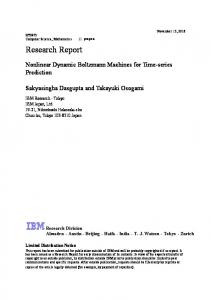
(a) LRBM
(b) LRBM
(c) SLRBM
Figure 1: Visualization of our locally connected generative models with lateral interaction. Dark nodes denote visible variables, light nodes hidden variables. The impact area of the hidden variable at the top left (in the SLRBM, for one mean field iteration) is depicted in light gray. Larger impact areas created through indirect (b) and direct (c) lateral interaction ensure global consistency in generated phantasies. have been applied to many domains, including text, speech, motion data, and images. The unsupervised learning procedure extracts features which are then used to generate a hidden representation of the input. By sampling from the distribution of hidden representations, one can then generate new data from the training distribution. In the most commonly used form, however, these models use global features, and do not take advantage of the topology of the input space. Especially when applied to image data, global features model long-range dependencies which are known to be weak in natural images (Huang and Mumford, 1999). We can observe that connectivity is problematic when we monitor learned features during RBM training. Such features are often presented in the literature (e.g. Hinton et al. 2006), where RBMs typically learned localized features. A small localized detail is attended on, while most of the filter has uniform weights. This is a result at the very late stages of the learning process, however. In early stages, the filters are global, similar to what one would expect from a PCA. We can conclude that much of the training time is wasted on learning that far-away pixels have little correlation. The obvious way to deal with this problem is to remove long-range parameters from the model, as shown in Figure 1a. The advantage of this 2
approach is two-fold: first, local connectivity serves as a prior that matches well to the topology of natural images, and second, the drastically reduced number of parameters makes learning on larger images feasible. The downside of local connectivity is that weaker long-distance interactions cannot be modelled at all. While local receptive fields are well-established in discriminative learning, their counterpart in the generative case, which we call “local impact area”, is not well understood. Generative models with local impact in the literature (e.g. Osindero and Hinton 2008; Welling et al. 2002; Roth and Black 2009; Hyv¨arinen and Hoyer 2001) do not try to sample whole images, only local patches. Breaking down the properties of RBM architectures is further complicated by the fact that RBMs are typically trained in an unsupervised way to maximize the likelihood of the training data, but then used as “pretrained” initialization of discriminative neural network training. In Section 7, we therefore analyze two questions (Q1) What do we gain? That is, how fast do local impact RBMs converge, when compared to dense models? (Q2) What do we loose? That is, how do local impact areas affect the representational power of the RBM? How well-suited for classification are the pre-trained RBMs? Obviously, when generating whole images from a local impact RBM, the architecture has no way to ensure that the generated images are globally consistent. For example, when the input distribution is images of Latin characters, local features are lines and crossings. Due to overlapping features, lines will be continued and crossings introduced as observed in the training images. However, the global statistics of characters is never represented, and therefore the architecture might generate Latin and Cyrillic characters with equal probability. To resolve the problem of global consistency, in this paper we investigate the capabilities of two Boltzmann-Machine-like graphical models: Stacks of local impact RBMs and RBMs with local lateral connections between the hidden units. We show how to avoid problems of generic Boltzmann machine learning in these models and attempt to answer the third question, (Q3) Can we recover from some of the negative effects of local impact areas using stacking or lateral connections? 3
We train our architectures on the well-known MNIST database of handwritten digits (LeCun et al., 1998). Our experiments demonstrate the efficiency of learning in locally connected RBMs. We also show how local impact areas can be efficiently implemented on Graphics Processing Units (GPU). As common in the deep learning literature (Bengio et al., 2008), the parameters learned in unsupervised training provide a good starting point for discriminative training of deep networks for classification. This also holds for RBMs with local impact areas. We show that when pre-training is used, the classification performance increases significantly in our models. Finally, we compare the classification performance of a model that exploits the image topology with a fully connected model. 2. Related Work There is a great body of work on generative models exploiting local structure (e.g. Osindero and Hinton 2008; Welling et al. 2002; Roth and Black 2009; Hyv¨arinen and Hoyer 2001), however, these models only provide generative models for image patches. While in principle these can also be used to generate whole images, this is not attempted – there is nothing in these methods ensuring global consistency. Consequently, the main application of these models is image denoising, that is, the correction of effects within patch range. We believe that for truly building generative models of images, it is essential to understand how the compatibility of neighbouring features can be assured. Related to the limited modelling capabilities discussed above, models such as Fields of Experts or Product of Student-t are “flat” in the sense that they are limited to a certain level of abstraction. To move beyond low-level vision, it is necessary to build a “deep” hierarchy of features. We believe that stacked RBMs and their variants pose a promising approach to higher-level feature modelling. Learned features are typically hard to evaluate. They are therefore often used for classification, directly, or after supervised fine-tuning. We also follow this approach in this paper, when other evaluation methods, such as determining or estimating the true log-likelihood of the data distribution, are infeasible. A well known supervised learning approach that makes use of the local structure of images is the convolutional neural network by LeCun et al. (1998). Another approach to exploit local structure for supervised training of recurrent networks has been suggested by Behnke (2003). LeCun’s ideas 4
where transfered to the field of generative graphical models by Lee et al. (2009) and Norouzi et al. (2009). None of these approaches have been used with pretraining. Their models, which employ weight sharing and max-pooling, discard global image statistics. Our model does not suffer from this restriction. For example, when training landscapes, our model would be able to learn, even on the lowest layer, that sky is usually depicted in the upper half of the image. To achieve globally consistent representations despite the local impact area, we make use of lateral connections between the latent variables. Such connections can be modelled in two ways, stacking and lateral interaction, discussed in the following paragraphs. Stacked RBMs as in Deep Belief Networks (DBN, Hinton et al. 2006) or Deep Boltzmann Machines (DBM, Salakhutdinov 2009) have an indirect lateral interaction between hidden variables through the features of the upper layer. Stacks of more than two RBMs, however, are not guaranteed to improve the data likelihood. In fact, even stacks of two RBMs do not improve a lower likelihood bound empirically (Salakhutdinov, 2009). Stacking locally connected RBMs, on the other hand, trivially yields larger effective impact areas for higher layers and thus can enforce more global constraints. A more direct way to model lateral interaction is to introduce pairwise potentials between observed or between latent variables. The former case, without restrictions to local impact areas, was studied by Osindero and Hinton (2008). However, this model mainly whitens the input, whereas our model ensures consistency of the hidden representations. Furthermore, Salakhutdinov (2008) trained general Boltzmann Machines (BMs) with dense lateral interactions between both observed and latent variables on small problems. Due to long training times, this general approach seems to be infeasible for larger problem sizes. Finally, it is not clear how to greedily train a stack BMs, as there would be two kinds of lateral interactions in each intermediate layer. 3. Background on Boltzmann Machines A BM is an undirected graphical model with binary observed variables v ∈ {0, 1}n (visible nodes) and latent variables h ∈ {0, 1}m (hidden nodes). The energy function of a BM is given by E(v, h, θ) = −vT W h − vT Iv − hT Lh − bT v − aT h, 5
(1)
where θ = (W, I, L, b, a) are the model parameters, namely pairwise visiblehidden, visible-visible and hidden-hidden interaction weights, respectively. The variables b and a are the biases of visible and hidden activation potentials. The diagonal elements of I and L are always zero. This yields a probability distribution p(v; θ) p(v; θ) =
1 ∗ 1 X −E(v,h,θ) p (v; θ) = e , Z(θ) Z(θ) h
where Z(θ) is the normalizing constant (partition function) and p∗ (·) denotes unnormalized probability. In RBMs, I and L are set to zero. Consequently, the conditional distributions p(v|h) and p(h|v) factorize completely. This makes exact inference of the respective posteriors possible. Their expected values are given by hvip(v) = σ(W h + b)
and
hhip(h) = σ(W v + b) .
(2)
Here, σ denotes element-wise application of the logistic sigmoid: σ(x) = (1 + exp(−x))−1 . The true gradient of the model is given by ∂ ln p(v) = hvhT i+ − hvhT i− . ∂W
(3)
Here, h·i+ and h·i− refer to the expected values with respect to the data distribution and the model distribution, respectively. In practice, however, Contrastive Divergence (CD, Hinton et al. 2006) is used to approximate the true parameter gradient by a Markov Chain Monte Carlo algorithm. The expected value of the data distribution is approximated in the “positive phase”, while the expected values of the model distribution are approximated in the “negative phase”. For CD in RBMs, h·i+ can be calculated in closed form, while h·i− is estimated using n steps of a Markov chain, started at the training data. Recently, Tieleman (2008) proposed a faster alternative to CD, called Persistent Contrastive Divergence (PCD), which employs a persistent Markov chain to approximate h·i− . This is done by maintaining a set of “fantasy particles” {(vF , hF )i } during the whole training. The chains are also governed by the transition operator in Equation (2) and are used to 6
calculate hvhT i− as the expected value with respect to the Markov chains hvF hTF i. We use PCD throughout this paper. When I is not zero, the model is called a Semi-Restricted Boltzmann Machine (SRBM, Osindero and Hinton 2008). This model can be trained with a variant of CD by approximating p(v|h) using a few damped mean field updates instead of many sequential rounds of Gibbs sampling. In SRBMs, lateral connections only play a role in the negative phase. We will later introduce our model, where lateral connections are used both in the positive and in the negative phase. RBMs can be stacked to build hierarchical models. The training of stacked models proceeds greedily layer-wise. After training an RBM, we calculate the expected values hhip(h|v) of its hidden variables given the training data. Keeping the parameters of the first RBM fixed, we can then train another RBM using hhip(h|v) as its input. 4. Local Impact Boltzmann Machines We now introduce two modifications to the classical RBM architectures described in Section 3. Stacks of Local Impact RBMs. Firstly, we restrict the impact area of each hidden node. To this end, we arrange the hidden nodes in multiple grids, called maps, each of which resembles the visible layer in its topology. As a result, each hidden node hj can be assigned a position pos(hj ) ∈ N2 in the input (pixel) coordinate system and a map map(hj ). This approach is similar to the common approach in convolutional neural networks (LeCun et al., 1998). We then allow wij to be non-zero only if | pos(vi ) − pos(hj )| < r for a small constant r, where pos(vi ) is the pixel coordinate of vi . In contrast to the convolutional procedure, we do not require the weights to be equal for all hidden units within one grid. We call this modification of the RBM the Local Impact RBM or LRBM. This model will help us to answer questions Q1 and Q2. Like RBMs, LRBMs can be stacked to yield deep feature hierarchies. Aside from the local impact areas, these models are not new. RBM stacks are typically trained greedily layer by layer to avoid problems with general Boltzmann machine learning (and then finetuned if desired, e.g. Salakhutdinov and Hinton 2009). However, they have been primarily introduced to generate more abstract features. In this work, stacked RBMs are trained to represent more 7
abstract features and more global statistics. Specifically, a high-level feature generated through stacking represents the statistics of low-level features which have a combined impact area wider than the impact area of a single low-level feature (Figure 1b). We show that straight-forward extension to a hierarchical feature organization helps to reduce the inconsistencies introduced through locality (question Q3) and is also helpful for classification (question Q2) LRBMs with Lateral Connections in the Hidden Layer. Similarly to stacking, direct (“lateral”) interactions between local features could provide an answer to question Q3. The lateral connections can ensure compatibility of activations and therefore enforce global consistency, as depicted in Figure 1c. We avoid the hardness of general Boltzmann machine training by demonstrating that for local lateral connections between local features, mean field updates are a feasible approach to learning. We allow lij to be non-zero if (i) i 6= j (lij is not a self-connection), (ii) map(hi ) = map(hj ) (i and j are on the same map) and (iii) | pos(hi ) − pos(hj )| < r0 (i and j are sufficiently close to each other). Here, r0 is a small constant denoting the size of the lateral neighbourhood. For simplicity, we assume L to be symmetric. Note that this assumption does not restrict the energy function in Equation (1), since E(v, h, θ) is symmetric in L. Learning in this model √ proceeds as follows. We initialize W with a normal distribution wij ∝ N (0, 1/ z), where z is the number of parameters directly influencing hj . L is initially set to zero. In the positive phase, the visible activations are given by the input and the hidden units form a conditional MRF with the biases of the hidden units determined by the visible units. To quickly minimize energy in the MRF, we resort to mean field inference and show in Section 7 that this choice is justified. The (damped) mean field updates are determined by h(0) = σ(W T v + b), h(k+1) = α h(k) + (1 − α) σ(W T v + b + LT h(k) ).
(4)
In the negative phase, we employ PCD to estimate hvhT i− . The state of the persistent Markov chain is denoted (vF , hF ). In the negative phase, we continue the persistent Markov chain by sampling vF from p(vF |hF ) = σ(W hF + a). 8
(k+1)
We then generate a new hidden state by sampling from p(hF |vF ), again estimated using mean field updates of Equation (4). We call this model LSRBM. Note that in contrast to SRBM (Osindero and Hinton 2008), the lateral connections play a crucial role in the positive phase. Avoiding Trivial Solutions. A common problem in training convolutional RBMs and convolutional neural networks is that the overcomplete representation of the visible nodes by the hidden nodes enables the filters to learn a trivial identity, where each filter has only one non-zero weight (Lee et al., 2009; Norouzi et al., 2009). Note that this is usually a bad solution, since examples not in the training data are also reconstructed perfectly. The above models therefore need an additional, heuristic sparsity bias. The methods proposed here do not suffer from this problem. First, we use PCD instead of CD-1 for training. While the weight update is zero in CD-1 learning when a training example can be perfectly reconstructed by the RBM, this is not the case for the PCD weight update in Equation (6), due to the PCD chain used. The particles (vF , hF ) of the PCD chain are sampled independently of the training data. Second, since in contrast to convolutional architectures no weight sharing is used, for a trivial solution to occur, all filters need to learn the identity separately, which is highly unlikely. 5. Finetuning LRBM Weights for Classification Tasks In many object recognition applications, it was shown that initializing the weights of a neural network with an unsupervised feature extraction algorithm improved the classification results. This procedure is commonly known as unsupervised pre-training and supervised fine-tuning in the deep learning literature. We use a locally connected neural network (LCNN, e. g. Uetz and Behnke 2009) for classification. Instead of randomly initializing the weights of the LCNN, we copy the LRBM weights into the LCNN after the LRBM was trained. Using the weights learned in a Local Impact Restricted Boltzmann Machine for initialization is straight-forward, since the arrangement of neurons in a LCNN matches the arrangement of hidden nodes in the LRBM. Finally, we connect an output layer to the LRBM by adding randomly initialized weights connecting each output (classification) unit to all units in the last layer of the LRBM. We can now proceed with the fine-tuning using gradient descent (back propagation of error) on the cross-entropy error function. First, the output 9
layer, which was not pre-trained, is adjusted while all other weights remain fixed. This prevents problems induced by large errors in the randomly initialized weights of the output layer destroying the pre-trained weights in earlier layers. After 30 epochs, the output weights have converged and we continue training the network as a whole. 6. GPU Acceleration As the 2D structure of the input maps well to the architecture of Graphics Processing Units (GPUs), we implemented the proposed architecture using the NVIDIA CUDA programming framework. To this end, we created a matrix library which, apart from common dense-matrix operations can operate on sparse matrices in diagonal format (DIA). These so-called stencil matrices can be used as weight matrices which are non-zero only at the local filter positions. This enables us to efficiently process large images, where the corresponding dense matrix W would not even fit in memory. Specifically, we implemented H ← WTV ,
V ← W H,
and
where H and V are dense matrices containing hidden/visible activations, respectively, and W is a LRBM weight matrix. Top-down and lateral connections have the same structure and therefore do not require additional specialization. Efficiency is further improved by processing 16 images in parallel. The gradient, ∆W ← V H T is calculated by multiplying all 16 × 16 submatrices of V and H, where the resulting submatrix is cut by one of the diagonals in ∆W . Our implementation, which focuses on ease of use by exporting all functionality to Python and seamlessly integrating with NumPy, gives an overall speedup of about 50 when compared to an optimized single CPU version. The code is available on our website2 . 7. Experimental Results In our experiments we analyze the effects of local impact areas and lateral interaction terms on RBMs. As a first step, we trained models with and without local impact areas on the MNIST database of handwritten digits (LeCun et al., 1998). The dataset is padded by a margin of four zero-pixels from 28 × 28 to 32 × 32 for convenient power-of-two scaling. 2
http://www.ais.uni-bonn.de/deep_learning/
10
(a) first layer
(b) second layer
(c) third layer
Figure 2: Visualization of indirect lateral interaction. We show activations associated with randomly selected hidden nodes in an LRBM, projected down from the respective layer.
log-prob. (nats) #Parameters
RBM-51
LRBM (12 × 12)
LRBM (7 × 7)
−125.58 400 819
−108.65 390 818
−109.95 270 058
Table 1: Test log-likelihood on MNIST for models with similar number of parameters: Densely connected RBM with 51 hidden nodes, Local Impact RBMs with varying impact area. For similar number of parameters, LRBMs achieve much better log-likelihood. We consider a stack of three LRBM and a (flat) LSRBM. The stack of three LRBMs has one map at the lowest layer, the input image. The layers above contain four, eight and 16 maps, respectively. Layer resolution is always set to half of the resolution of the layer below, resulting in map sizes of 32×32, 16 × 16, 8 × 8 and 4 × 4. The size of the local impact areas is 12 × 12 in the lowest layer, 10 × 10 in the second layer and 8 × 8 in the third layer. Since the resolution of the third layer is 8 × 8 as well, the last LRBM in the stack is a common, densely connected RBM. The LSRBM also has a local impact area of 12 × 12, but the size of the window for lateral connections is 15 × 15. For damping in Equation (4) we use α = 0.2 as taken from Osindero and Hinton (2008). 7.1. Data Modeling To evaluate the power of the LRBM as a generative model, we approximate the likelihood assigned to the test data under these models using Annealed Importance Sampling (AIS, Salakhutdinov 2009). The likelihood is measured 11
Network
With Pretraining
Without Pretraining
1.49 1.39
1.63 1.58
Fully connected LCNN
Table 2: MNIST classification error in percent in “nats”, meaning the natural logarithm of the unit-less probabilities. We compare the LRBM to a standard RBM model with 51 hidden units, so that it has a slightly higher number of parameters than the locally connected model with a hidden layer consisting of two maps of size 16 × 16, and an impact area of size 12 × 12. The results are summarized in Table 1. The locally connected model had a test log-likelihood of −108.65 nats whereas the standard RBM had a test log-likelihood of −125.58 nats, showing a clear advantage of our model. For comparison, a fully connected RBM with as many hidden units as the local model achieves a test log-likelihood of −101.69 nats. However, this model has eight times more parameters. As the number of parameters scales quadratically with the image size, such dense matrices will not be an alternative for larger images. Further decreasing the number of parameters by reducing the size of the impact area by factor of 0.65 does not significantly reduce the test log-likelihood (LRBM 7 × 7, −109.95 nats). We can therefore answer the first part of question Q2: For a given number of parameters, the local model performs significantly better than the dense model in terms of data likelihood. However, since dense models were shown to learn local properties of the dataset and we simply force connections to be local only, it is not clear why local models perform worse than large dense models in the first place. We hypothesize that this loss stems from the fact that the LRBM is not able to ensure global consistency. In Section 7.4, we investigate possible solutions for this effect. 7.2. Classification In order to assess the fitness of the extracted features for classification (second part of question Q2), we train a locally connected neural network, as described in Section 5, starting from the weights learned in the stack of LRBMs. Since we aim at comparing different learning methods, we do not augment the training set with deformed versions of the training data, which generally guarantees performance improvements (e. g. LeCun et al. 1998). We want to show the advantage that LRBMs have over (dense) RBMs. 12
For this purpose, we compare our approach with a vanilla fully connected neural network, a locally connected network without pre-training and a fully connected neural network, pre-trained with a standard RBM. In all cases, the network output is represented by a one-out-of-ten code. Using a parameter scan on a validation set, we found that the best result for using a vanilla neural network are achieved with one hidden layer containing 400 neurons. Using this setup, we obtained a test error of 1.63%, which serves as a baseline. For this task, we replace the topmost layer of the stack of LRBMs with ten neurons of the output layer. These neurons are fully connected to the second hidden layer. Table 2 summarizes the obtained results. For selecting the LRBM setup we also performed a parameter scan. Using a validation set we selected a model with one hidden layer and 4 maps with a resolution of 28 × 28. From the table it is clear that locally connected networks have an advantage over fully connected networks. This finding is expected and indicates that local connectivity is indeed a useful prior for images. We also find that pretraining the neural networks improves performance. This is not only true for the fully connected network, as was repeatedly found in the literature, but also for the LCNN. We can therefore conclude that the restriction of connectivity enforced by local impact areas helps networks to analyze images. However, it determines the resulting filters only so much that they can still profit from unsupervised pretraining. In conclusion, the answer of the second part of question Q2 is that LRBMs are well suited for classification of images when they are used as weightinitializations for locally connected neural networks in conformance with standard deep learning methods. 7.3. Effectiveness of Mean Field Updates for Inference The method used to learn lateral connections, as explained above, is similar to the one used in Osindero and Hinton (2008) where it was applied successfully to learning lateral connections between visible nodes. Since in this work, it is used to learn lateral connections between hidden nodes, we performed experiments to justify its use. First, we calculated the energy of states inferred with both sequential Gibbs sampling and mean field updates E(v, h, θ) = −vT W h − hT Lh − bT v − aT h,
(5)
of a one layer LRBM. Gibbs updates where run until the mean energy converged, since this indicates arriving at the stationary distribution. Both before 13
and after training, the distribution over energies on the training set using sequential Gibbs sampling and mean field updates where indistinguishable. These results suggest that mean field updates find states that are as probable as those found by running sequential Gibbs updates. Since we are interested in the approximation of hhT i− mainly for calculating the weight updates during learning, we also compared weight updates obtained by using mean field updates with those obtained by Gibbs sampling. We measured the magnitude k∆W k2 of the updates ∆W = hvhT i+ − hvhT i− .
(6)
Let ∆WG be the update when sequential Gibbs sampling is used to approximate hvhT i− and ∆WM be the update if the mean field method is used. We compare k∆WG k2 and k∆WG − ∆WM k2 to judge the impact of the mean field method on the calculation of the update ∆W . Using different random optimizations and different model parameters we consistently observed that k∆WG − ∆WM k2 is at most 13 k∆WG k2 . From this we conclude that our learning algorithm does not significantly change the direction of the weight updates compared with a more exact but more time consuming method. 7.4. Qualitative Analysis Both RBMs and LRBMs model local features, LRBMs do so directly, RBMs only after they have learned that only close-by pixels are correlated. LRBMs would be the logical choice, then, if the LRBM model would not have one central deficiency. In dense models, long-range interactions are weak, but represented nevertheless. LRBMs cannot represent them at all. We therefore evaluate the influence of direct and indirect lateral interactions in the generative context, to recover global consistency and to answer question Q3. To this end, we visualized filters and fantasies generated by LRBM and LSRBM. The images in Figure 2 show weights in an LRBM with three layers. In the first image, filters of the lowest hidden layer are projected down to the visible layer. We observe that small parts of lines and line-endings are learned. The second and third images display filters from the second and third hidden layer, projected down to the visible layer. These filters are clearly more global. With their size, the size of the recognized structure increases as well. The images in Figure 3 visualize direct lateral interactions in an LSRBM. The first row shows randomly selected filters hj of the first hidden layer, while 14
Figure 3: Visualization of direct lateral interaction in LSRBM. The first row shows top-down filters, the second row shows lateral connections projected to visible layer. The lateral filters learned to implicitly extend the top-down filter at the same position, thereby enforcing consistency between hidden activations. the second row depicts a linear combination of all other filters hi , weighted by their pairwise potential lij . Note that hj does not contribute to this sum, since ljj = 0. We observe that through lateral interaction the filter is not only replicated, it is even extended beyond its impact area to a more global feature. Figure 4 shows fantasies generated by LSRBM and a stack of LRBMs. Markov chains for fantasies were started using binary noise in the visible layer. Each Markov chain ran for 300 steps, followed by 100 mean field updates. It is clear that fantasies produced by a single-layer LRBM are only locally consistent and one can observe that stacking gradually improves global consistency. Lateral connections in the hidden layer significantly improve consistency even for a flat model. We also observed that LSRBM and stacked models need less iterations of the Markov chain to converge to the model distribution (data not shown). These findings strongly support our initial claim that lateral interaction compensates for the negative effects of the local impact areas, which answers question Q3 to the affirmative. 8. Conclusions In this work, we present a novel variation of the Restricted Boltzmann Machine for image data, featuring only local interactions between visible and hidden nodes. This structure matches well with the topology of images and reflects the observation that long-range interactions are scarce in images, anyway. In contrast to to dense RBMs, locally connected RBMs can be scaled to realistic image sizes. 15
(a) LSRBM, 1 layer
(b) LRBM, 1 layer
(c) LRBM, 2 layers
(d) LRBM, 3 layers
Figure 4: Fantasies generated by our models from random noise. Lateral connections as well as stacking enforce global consistency. We analyze the local models and find that they perform very well when compared to dense RBMs with similar number of parameters in terms of data likelihood. As common in the deep learning literature, we use the learned RBMs as initializations of deep discriminative, and in our case local, neural networks. The results show that the local RBMs can also improve classification performance, so that we believe this widely used technique can be adopted to larger problems where dense RBMs are not an option anymore. While learning in this model is fast and few parameters yield comparably good data probabilities and classification performance, the model does not enforce global consistency constraints when sampling fantasies from the model. We showed that this effect can be at least partially compensated for by adding lateral interactions between the latent variables, which we model directly by pairwise potentials or indirectly through stacking. Due to the small number of parameters and its computational efficiency, our architecture has the potential to model images of a much larger size than commonly used forms of RBMs. We are currently working towards this goal. 9. Acknowledgements We would like to thank the anonymous reviewers for valuable suggestions for improvement on earlier versions of this paper. References Behnke, S., 2003. Hierarchical neural networks for image interpretation. Lecture notes in Computer Science Vol. 2766 Springer-Verlag. 16
Bengio, Y., Lamblin, P., Popovici, D., Larochelle, H., 2008. Greedy layer-wise training of deep networks. In: Advances in Neural Information Processing Systems (NIPS) 20. pp. 841–848. Hinton, G., 2002. Training Products of Experts by Minimizing Contrastive Divergence. Neural Computation 14 (8), 1771–1800. Hinton, G., Osindero, S., Teh, W., 2006. A fast learning algorithm for deep belief nets. Neural Computation 18 (7), 1527–1554. Huang, J., Mumford, D., 1999. Statistics of natural images and models. In: IEEE Conference on Computer Vision and Pattern Recognition (CVPR). pp. 1541–1547. Hyv¨arinen, A., Hoyer, P., 2001. A two-layer sparse coding model learns simple and complex cell receptive fields and topography from natural images. Journal on Vision Research 41 (18), 2413–2423. LeCun, Y., Bottou, L., Bengio, Y., Haffner, P., 1998. Gradient-based learning applied to document recognition. Proceedings of the IEEE 86 (11), 2278– 2324. Lee, H., Grosse, R., Ranganath, R., Ng, Y., 2009. Convolutional deep belief networks for scalable unsupervised learning of hierarchical representations. In: International Conference on Machine Learning (ICML). pp. 609–616. Norouzi, M., Ranjbar, M., Mori, G., 2009. Stacks of Convolutional Restricted Boltzmann Machines for Shift-Invariant Feature Learning. In: IEEE Conference on Computer Vision and Pattern Recognition (CVPR). IEEE, pp. 2735–2742. Osindero, S., Hinton, G., 2008. Modeling image patches with a directed hierarchy of Markov random fields. Advances in Neural Information Processing Systems (NIPS) 20, 1121–1128. Roth, S., Black, M., 2009. Fields of experts. International Journal of Computer Vision (IJCV) 82 (2), 205–229. Salakhutdinov, R., 2008. Learning and evaluating Boltzmann machines. Tech. rep., University of Toronto.
17
Salakhutdinov, R., 2009. Learning Deep Generative Models. Ph.D. thesis, University of Toronto. Salakhutdinov, R., Hinton, G., 2009. Deep Boltzmann Machines. In: Converence on Artificial Intelligence and Statistics (AIStats). Vol. 5. pp. 448–455. Smolensky, P., 1986. Information processing in dynamical systems: Foundations of harmony theory. In: Rumelhart, D., McClelland, J. (Eds.), Parallel Distributed Processing. Vol. 1. MIT Press, Cambridge, Ch. 6, pp. 194–281. Tieleman, T., 2008. Training restricted Boltzmann machines using approximations to the likelihood gradient. In: International Conference on Machine Learning (ICML). pp. 1064–1071. Uetz, R., Behnke, S., 2009. Large-scale Object Recognition with CUDAaccelerated hierarchical neural networks. In: IEEE International Conference on Intelligent Computing and Intelligent Systems. pp. 536–541. Welling, M., Hinton, G., Osindero, S., 2002. Learning sparse topographic representations with products of student-t distributions. In: Advances in Neural Information Processing Systems (NIPS). pp. 1359–1366.
18