[PAR86] A. C. Parker, J. Pizarro, and M. Mlinar, "MAHA: A program for datapath synthesis",. Proceedings 22nd DAC, pp. 461-466, June 1986. [PAU89] P. G. ...
Exploiting Scheduling Freedom in Controller Synthesis* John A. Nestor and Vili Tamas Department of Electrical and Computer Engineering Illinois Institute of Technology Chicago, Illinois 60616 Abstract The partial ordering provided by a control-data flow graph (CDFG) gives synthesis tools flexibility in ordering the operations in a behavioral description. This flexibility is often used to reduce datapath cost, but is seldom used to reduce controller cost. This paper describes work in progress that is developing a representation of scheduling flexibility in controllers and a procedure for exploiting this flexibility to reduce the cost of controller implementations generated by a high-level synthesis system. 1. Introduction Most approaches to high-level synthesis [MCF90] work from a control-data flow graph (CDFG) representation that provides a partial ordering of operations in the original behavioral description. During synthesis, this partial ordering provides great flexibility in scheduling operations that can be used to reduce the cost of the implementation. Many scheduling algorithms (e.g. [PAR86, PAN87, PAU89, NES90]) exploit this freedom to reduce datapath cost. However, only limited efforts have been made to use scheduling freedom to reduce controller cost, especially when the controller is implemented as a single finite state machine (FSM). One reason for this is that few synthesis tools use controller specifications that can express scheduling freedom. Exceptions include the USC ADAM representation [HAY89], the Stanford Hercules/Hebe [KU90,KU91] system, and the Princeton PUBSS system [WOL90,WOL91]. The ADAM representation maintains scheduling freedom for use during control synthesis. However the current controller synthesis tool does not exploit this information. Hercules/Hebe [KU91] optimizes the cost of a set of interacting controllers using resynchronization of operations but does not address the problem of reducing the cost of a single FSM controller. The PUBSS [WOL91] system exploits scheduling freedom to minimize the number of states in the controller FSM, but does not directly consider the effect of scheduling on implementation cost. This paper describes a new effort to exploit scheduling freedom when generating controllers from scheduled and allocated CDFGs. This approach is based on a representation of controllers as finite state machines in which the clock-cycle level timing of * This research was supported in part by NSF Grant MIP-9010406.
1
outputs is loosely specified using a partial ordering of output events. We present a branch and bound algorithm for scheduling output events to minimize the cost of a two-level PLAstyle implementation and show how such controller descriptions can be extracted from a scheduled and allocated CDFG. While this procedure is primarily intended for use in the controller synthesis phase of a high-level synthesis system, it may also be used in other situations where controller specifications may contain scheduling flexibility. For example, it may be used to optimize the control program for a previously-designed datapath in a task analogous to microcode compaction [DAV81] but targeted towards FSM controllers. In addition, it could be used as a synthesis procedure for FSM-based interface circuits [BOR87] that are specified in timing-diagram form. This paper is organized as follows: Section 2 describes the details of the representation, while Section 3 describes the scheduling procedure for minimizing implementation cost. Section 4 describes how controller specifications are extracted from a scheduled and allocated CDFG. Section 5 describes the current status of the project, and Section 6 provides conclusions and a discussion of future work. 2. Describing Scheduling Freedom in Finite State Machines In our approach, scheduling flexibility is specified in FSM controllers using a representation called Output Transition Graphs (OTGs). An OTG represents the behavior of a controller without completely specifying the exact timing of transitions in output values. It is similar in structure to Borriello's event graph [BOR87] and Wolf's Behavioral Finite State Machine (BFSM) representation [WOL91], but is more directly descended from the CDFG representation used in many high-level synthesis systems [MCF90]. In the OTG representation, a controller specification describes a Moore-style FSM with imprecise timing using a collection of graphs, where each graph represents a basic block in the controller (i.e. a sequence of one or more states with a single entry point and a single exit point). The overall representation is a tuple: where I represents the set of inputs, O represents the set of outputs, B represents the set of basic blocks {b1,b2, ..., b|B|}, and T represents the set of transitions {t1,t2, ..., t|T|} between basic blocks. Each transition has an associated input condition that specifies the conditions under which the transition occurs. Note that this specification is quite similar to traditional representations for FSMs (e.g. [DEV87]), except that each block represents a straight-line sequence of states rather than an individual state. Within a block, all transitions between states are unconditional except for the final state. Transitions from the final state are specified by the block transitions. Following the terminology used in highlevel synthesis, we will often refer the states within a block as the control steps of that block.
2
Each block bi ∈ B represents the behavior of a straight-line sequence of states in which the timing of output transitions is imprecisely specified. This is accomplished using a directed graph G(V,E) consisting of vertices (nodes) V = {vsrc,v1, v2, ..., vn,vsink} and edges E = {eij | vi , vj ∈V }. Vertices in the graph include a single source and sink node, dummy nodes that are used to tie together groups of operations, and output event nodes that represent transitions in output value. Each output event specifies a controller output vi.output and output value vi.value. When an output event is "executed", the output takes on the specified value in the in that state and holds that value in subsequent states until another event with the same output is encountered. A block is scheduled by assigning to each node vi an integer control step value between 0 and L+1, where L is the length of the schedule of that block. We will refer to the scheduled position of vi as vi.step. By convention, the source node vsrc of each graph is always scheduled in control step 0 (zero), while the sink node vsink is always scheduled in step L+1. All other nodes are scheduled in steps 1 through L, and a scheduled graph represents L states in the resulting FSM implementation. Edges act as ordering and timing constraints that partially specify scheduling of event nodes. Each edge represents an inequality relationship between the scheduled positions of vertices. Minimum constraints between two vertices vi and vj are specified using an edge weight eij.min, which represents the inequality: vj.step ≥ vi.step + eij.min Similarly, maximum constraints between two vertices vi and vj are specified using an edge weight eij.max, which represents the inequality: vj.step ≤ vi.step + eij.max All edge weights are specified in terms of control steps (clock cycles). Precedence constraints are usually represented by constraint weights of 1 or 0, while timing constraints use weights equal to the number of control steps of the constraint. The length of a block schedule can be constrained by a constraint edge between the source and sink vertices that is weighted with the desired length plus one. If no such edge is present, then the schedule length is set to the shortest length that satisfies all other constraints. Event vertices that are associated with the same output are subject to precedence constraints which specify an ordering (but not precise scheduling) of these events. This guarantees that the order of output values in the initial specification is preserved but allows variation in the exact time when the output takes on these values. These constraints are represented by edges as before, but it is also convenient to refer to them as the predecessor and successor events of vi: vi.prev and vi.next. Event vertices that are associated with the same output may be scheduled in the same control step (i.e. "chained" [PAN87]) if permitted by constraints. In this case, the last event that is scheduled in the step (in order
3
of precedence) overrides all other events and specifies the value that the output will take on. However, it is up to the user to make sure that this results in a consistent specification. Initial output values may be specified in a block in two ways. First, output events may be constrained to be scheduled in step 1 using constraints from the source vertex. Since these nodes will always be scheduled in the first step, these specify a known value at the beginning of the block. Second, output values may be derived from previously executed blocks. However, since there is currently no support in the OTG representation for conditional outputs, this value must be consistent when a block has more than one entry point. For example, when two paths of execution lead into a block both paths must specify the same output value (i.e. both 0 or both 1 only). Data-flow analysis is used to detect and report inconsistent output values. If these values occur, they are reported as an error but are treated as don't cares in the controller specification. Figure 1 shows an example of a simple output transition graph that describes a looselyspecifed sequence of outputs in a single basic block. Value transitions on output X are specified by two event nodes, which specify that X first takes on the value 1, then the value 0. Similarly, value transitions are specified for output Y by three nodes, which specify that Y first takes on the value 0, then 1, then 0. Timing constraint edges between these nodes specify ordering relationships, and constraints from the source node to the initial events consistently specify initial values at the beginning of the block. Another timing constraint between the source and sink nodes fixes separation of the source and sink at 5 control steps and so fixes the schedule length at 4 control steps. Finally, a single block transition specifies an infinite loop.
src
X
=1
=1
1
Y 0 ≥1
≥1 =5
0
1 ≥1
≥1
0 snk
- (unconditional)
Figure 1 - OTG Example Finding a schedule that meets timing and ordering constraints can be viewed as a constraint solution problem similar to that found in one-dimensional layout compaction [LIA83,BUR86]. This problem can be solved using constraint solution techniques that start with all vertices scheduled in step 0 and iteratively correct individual constraint
4
violations by moving vertices into later control steps until all constraints are satisfied. This approach has been applied in high-level synthesis [KU90,NES90] and results in an "as soon as possible" (ASAP) schedule that meets all timing and ordering constraints. An "as late as possible" (ALAP) schedule can be found in a similar way placing all nodes at the end of the schedule and moving nodes to previous control steps until all constraints are satisfied. The ASAP and ALAP schedules are usually not the best schedules with respect to implementation cost. However, they are quite useful because they characterize the range of steps in which each vertex may be scheduled. This use of this property is described in the next section. Figure 2 shows three possible schedules for the OTG of Figure 1: the ASAP schedule, the ALAP schedule, and the schedule which results in the lowest implementation cost. In addition, it shows the implementation of these schedules in two-level logic assuming that control steps 1-4 are assigned state codes "00","01","11", and "10", respectively. Each implementation is shown as the initial logic cover for the schedule and the minimized cover that results after logic minimization using Espresso [RUD87]. After logic minimization, the ASAP and ALAP schedules both require 3 product terms. However, the third schedule only requires two product terms. The next section describes a systematic way to find and exploit such product term savings, as well as cost savings due to column compaction. ASAP Schedule
Block B1 0
Block B1
src
X
0
=5
0
1
≥1
4 5
=
1
1
≥1
0
≥1 2
=5
≥1
=5
1 ≥1
3
1
0
≥1 4
0
≥1 4
0
≥1
5 snk
≥1
0 ≥1
5
snk
- (unconditional)
2 4 0110 1101 1000 0000
Y =1
0
3
0
.i .o 00 01 11 10
X
≥1
3
Initial Logic Cover
src
=1
≥1 2
0
Y
1
1
≥1
≥1
Block B1
X =1
1
Best Schedule
src
=1
≥1 2
0
Y =1
1
ALAP Schedule
Minimized Logic Cover
.i .o -1 00 01
2 4 1000 0110 0101
snk
- (unconditional) Initial Logic Cover
.i .o 00 01 11 10
Minimized Logic Cover
2 4 0110 1110 1011 0000
.i .o -1 11 0-
2 4 1000 0011 0110
- (unconditional) Initial Logic Cover
.i .o 00 01 11 10
2 4 0110 1111 1001 0000
Figure 2 - Implementations of Three Schedules
5
Minimized Logic Cover
.i .o -1 0-
2 4 1001 0110
3. Scheduling Output Transition Graphs Scheduling of output transition graphs is very similar to scheduling CDFG nodes in high-level synthesis. This section discusses how scheduling techniques developed in highlevel synthesis can be applied to scheduling Output Transition Graphs. 3.1 Scheduling Overview Output transition graphs are scheduled by assigning nodes in each block to control steps that represent states in each block. This assignment must be done in a way that satisfies the constraints represented by the edges between nodes. A partial schedule is formed when some but not all nodes are assigned to control steps. A complete schedule is formed when all nodes are assigned to steps. The ASAP and ALAP schedules of a graph represent the earliest and latest that each node in a graph may be scheduled. In an unscheduled graph with a maximum length constraint, the ASAP and ALAP schedules specify the range of control steps into which a node may be scheduled. This interval is often called the time frame of a node [PAU89]. The size of a node's time frame is often referred to as then node's freedom [PAR86] or mobility [PAN87]. When a node is scheduled, its assignment to a particular control step will limit the time frames of other nodes that are related to the scheduled node. Each time a node is scheduled into a control step, the ASAP and ALAP positions of related nodes will move closer together. Partial schedules can be characterized by the positions of the unscheduled nodes and the time frames of the unscheduled nodes. As more nodes are scheduled, the time frames of the remaining nodes are restricted until often a node can be scheduled only in a single control step. We refer to these nodes as implicitly scheduled nodes Several scheduling techniques in high-level synthesis use time frames to guide the scheduling process (e.g. [PAR86,PAN87,PAU89]). Starting with a completely unscheduled graph, they evaluate the time frames and choose a node based on some prediction of effect on schedule cost. However, these approaches concentrate on the cost of the datapath and do not consider the effect of scheduling decisions on controller cost. 3.2 Scheduling to Optimize Controller Cost Scheduling freedom in a controller specification such as the OTG representation can be used to optimize controller cost by adapting scheduling methods from high-level synthesis to controller synthesis. However, different methods are needed to guide the scheduling process. Specifically, some measure of schedule cost must be developed. A straightforward cost measure is estimated implementation cost for a PLA implementation. Assuming that state assignment is already performed, a complete schedule specifies output values in every state in the form of a multiple-output, two-level logic function that consists of a number of inputs I, outputs O, and product terms P. While the number of inputs is fixed, the number of product terms and outputs can often be reduced. 6
Specifically, a fast heuristic logic minimizer such as Espresso [RUD87] can reduce the number of product terms P to P', and a column compaction procedure [WEI87] can combine output columns to reduce the number of outputs O to O'. After these steps, implementation cost for a PLA implementation can be estimated as: COST = (2*I + O')*P' An obvious approach, then, would be to evaluate the cost of every possible output schedule using this method and select the best implementation. However, the number of schedules that must be evaluated makes this approach infeasible. The approach used here is to develop an evaluation function that works with partial schedules and returns a lower bound on the implementation cost of all possible schedules that would result from that partial schedule. This function can then be used to guide a branch-and-bound approach to scheduling and substantially reduces the number of evaluations that must take place. 3 . 3 Evaluating Partial Schedules A lower-bound function can be developed by examining the effect of uncertainty of output values in a partial schedule on a predicted implementation cost. However, we must first characterize the conditions under which values are uncertain in a partial schedule. In a complete schedule, the value of every output is known in every control step. Specifically, the value of an output in a control step is defined by: value(output,step) = vi.value, vi ∈ V | output = vi.output ∧ step ≥ vi.step ∧ step < vi.next.step In a partial schedule, the exact position of unscheduled output events is not known. However, since it is known that the event must fall between its ASAP and ALAP schedules, values can at least be determined when a control step falls in or after the ALAP position of one output event and before the ASAP position of the next output event. Thus for a partial schedule,
v i.valueּifּ∃ּv iּ∈ ּVּ|ּoutputּ=ּv i.outputּ∧ּ stepּ>=ּv i.alapּ∧ּstepּ