Université de Saint-Etienne, Jean Monnet, F-42000, Saint-Etienne, France. Optical interferometers provide multiple wavelength measurements. In order.
Exploiting spatial sparsity for multi-wavelength imaging in optical interferometry ´ Eric Thi´ ebaut1 , Ferr´ eol Soulez1 and Lo¨ıc Denis2 Universit´e de Lyon, Lyon, F-69003, France; Universit´e Lyon 1, Observatoire de Lyon, 9 avenue Charles Andr´e, Saint-Genis Laval, F-69230, France; CNRS, UMR 5574, ´ Centre de Recherche Astrophysique de Lyon; Ecole Normale Sup´erieure de Lyon, Lyon, F-69007, France. 2 Universit´e de Lyon, F-42023, Saint-Etienne, France, CNRS, UMR5516, Laboratoire Hubert Curien, F-42000, Saint-Etienne, France, Universit´e de Saint-Etienne, Jean Monnet, F-42000, Saint-Etienne, France.
arXiv:1209.2362v2 [astro-ph.IM] 18 Dec 2012
1
Optical interferometers provide multiple wavelength measurements. In order to fully exploit the spectral and spatial resolution of these instruments, new algorithms for image reconstruction have to be developed. Early attempts to deal with multi-chromatic interferometric data have consisted in recovering a gray image of the object or independent monochromatic images in some spectral bandwidths. The main challenge is now to recover the full 3-D (spatio-spectral) brightness distribution of the astronomical target given all the available data. We describe a new approach to implement multi-wavelength image reconstruction in the case where the observed scene is a collection of point-like sources. We show the gain in image quality (both spatially and spectrally) achieved by globally taking into account all the data instead of dealing with independent spectral slices. This is achieved thanks to a regularization which favors spatial sparsity and spectral grouping of the sources. Since the objective function is not differentiable, we had to develop a specialized optimization algorithm which also accounts for non-negativity of the brightness distribution. c 2012 Optical Society of America
OCIS codes: 100.3175, 100.3190, 100.4145 1.
Introduction
The objective of stellar interferometric imaging is to recover an approximation of the specific brightness distribution Iλ (θ) of observed astronomical objects given measurements providing incomplete samples of the spatial Fourier transform of Iλ (θ). Reconstruction of a monochromatic image from optical interferometry data is a challenging task which has been the subject of fruitful research and resulted in various algorithms (e.g., Mira [1], Bsmem [2, 3], Wisard [4], the building-block method [5]). When dealing with multi-spectral data, a first possibility is to process each wavelength independently and reconstruct a monochromatic image for each subset of measurements from a given spectral channel. For instance, this is what have been done by le Bouquin et al. [6] for the multi-spectral images of the Mira star T Lep. Another possibility is to exploit some assumed spectral continuity of Iλ (θ) and process the multi-spectral data globally to reconstruct an approximation of the 3-D distribution Iλ (θ). This computationally more challenging approach can potentially lead to better reconstructions. Significant improvements have been shown when following such spatio-spectral processing in the context of integral field spectral spectroscopy [7–9]. This paper describes a method to jointly reconstruct multi-spectral optical interferometric data. In order to simplify the problem, we restricted our
study to the cases where the complex visibilities are observed and where the observed scene is a collection of point-like sources. This correspond, for instance, to the science case of the instrument Gravity which will be installed at the Very Large Telescope Interferometer (VLTI) to carry out astrometry with absolute phase reference of stars in the galactic center or in globular clusters [10]. In some sense, this latter assumption makes our algorithm a successor of the Clean algorithm [11, 12] and the building-block method [5] developed for recovering monochromatic images from radio and optical interferometric data respectively. The Clean algorithm have been proposed for the processing of Gravity interferometric data [13] but only considering “gray” data and not more than three stars in the field of view. In addition to processing multi-variate data, we also introduce the explicit minimization of a non-differentiable regularization term so as to favor spatial sparsity of the reconstructed brightness distribution in a way which is known to be more efficient [14, 15] than greedy algorithms like Clean [16] or the building-block method [5]. The method presented in this paper improves over early developments presented as an invited paper at the 2012 SPIE Conf. on Astronomical Telescopes & Instrumentation in Amsterdam[17]. Our paper is organized as follows: we first summarize the inverse approach for image reconstruction from interferometric data and discuss various possibilities to
2 impose spatial sparsity, we then detail our algorithm for minimizing the objective function; finally we present some results on simulated data and discuss the advantages of our approach. 2.
Method
A.
General principle of image reconstruction
yp,m,` = (H · x)p,m,` + ep,m,` X = Hp,m,n,` xn,` + ep,m,` , n
Following an inverse approach, we state image reconstruction as a constrained optimization problem [18]: x+ = arg min {fdata (x) + µ fprior (x)}
(1)
x∈X
where x ∈ R|x| are the sought image parameters, |x| = Card(x) is the number of parameters, X ⊂ R|x| is the subset of feasible parameters, fdata (x) is a data fitting term which enforces agreement of the model with the measurements y ∈ R|y| , fprior (x) is a regularization term and µ > 0 is a so-called hyper-parameter used to tune the relative weight of the regularization. Following a Bayesian interpretation, fdata is the opposite of the loglikelihood of the measurements, fprior is the opposite of the log of the prior distribution of the parameters, and x+ defines the maximum a posteriori (MAP) estimate. Constraining the solution to belong to the feasible set X is a mean to impose strict constraints such as the nonnegativity: X = {x ∈ Rn : x ≥ 0}
(2)
where the inequality x ≥ 0 is to be taken element-wise. B.
with complex arithmetic. In our framework, the model of the data is affine:
Direct model and likelihood
In this study, we assume that the optical interferometric data consist in Fourier transform of the brightness distribution Iˆλ (ν) measured for a finite set of spatial frequencies ν = B/λ with B the interferometric baseline (projected in a plane perpendicular to the line of sight) and λ the wavelength [19]. The most practical representation of a multi-variate distribution such as Iλ (θ) by a finite number of parameters x consists in sampling Iλ (θ) separately along its spatial and spectral dimensions. The image parameters are then: xn,` ≈ Iλ` (θ n )
(3)
for λ` ∈ W the list of sampled wavelengths and θ n ∈ A the list of angular directions, the so-called pixels. For the sake of notational simplicity, we use the same wavelengths in W as the ones of the data spectral channels and we denote by yp,m,` the real (p = 1) or imaginary (p = 2) part of the complex visibility obtained with mth baseline in `th spectral channel. This notation is intended to clarify the equations and does not impose or assume that all baselines have been observed in all spectral channels. By considering that complex numbers are just pairs of real values, our notation also avoids dealing
(4)
where the term e accounts for noise and modeling approximations. Formally, the coefficients of the operator H are given by [19]: ( + cos(θ > n · B m /λ` ) for p = 1 Hp,m,n,` = (5) > − sin(θ n · B m /λ` ) for p = 2 with B m the mth observed baseline and θ > n·B m the usual scalar product between B m and θ n . At least because of the strict constraints imposed by the feasible set X, solving the image reconstruction problem in Eq. (1) must be carried out by an iterative algorithm. Owing to the size of the problem, a fast version of H has to be implemented. First, we note that the model is separable along the spectral dimension (using a conventional matrix representation, H would have a block diagonal structure): y ` = H` · x` + e` ,
(6)
where the index ` denotes the sub-vector or the suboperator restricted to the coefficients corresponding to the `th spectral channel. With the generalization of multi-processor computers or multi-core processors, this property of the operator H may be easily exploited to parallelize the code to apply H (or its adjoint H> ) to a given argument. Second, an algorithm such as the nonuniform fast Fourier transform (NU-FFT) [20] can be implemented to speed up the computations by approximating the operator H` by: H` ≈ R` · F · S
(7)
where F is the discrete Fourier transform (DFT), R` interpolates the discrete spatial frequencies resulting from the DFT at the frequencies observed in `th channel and S is a zero-padding and apodizing operator. Zeropadding improves the accuracy of the approximation, while apodization pre-compensates for the convolution by the interpolation kernel used in R` [20]. Note that only the interpolation in the Fourier domain R` depends on the spectral channel. In NU-FFT, S is diagonal, R` is very sparse and F is implemented by a fast Fourier transform (FFT) algorithm, thus the approximation in Eq. (7) is very fast to compute. Assuming Gaussian noise distribution, the likelihood term writes: fdata (x) =
1 (H · x − y)> · W · (H · x − y) 2
(8)
where W ∈ R|y|×|y| is a statistical weighting matrix; in principle, W is the inverse of the covariance matrix of the measurements: W = Cov(y)−1 .
3 C.
Regularization based on spatial sparsity
Due to the voids in the spatial frequencies covered by the observations, the constraints provided by the data alone do not suffice to define a unique image. The prior constraints imposed by fprior (x) are then required to help choosing a unique solution among all the images that are compatible with the measurements. In this paper, we focus on a particular type of astronomical targets which consist in a number of point-like sources with different spectral energy distributions. This includes the case of multiple stars, globular clusters, or groups of stars as observed in the center of our galaxy. For such objects, the most effective means to regularize the problem is to favor spatially sparse distributions, i.e. images with as few sources as possible on a dark background. In this section, we derive expressions of the regularization term fprior (x) suitable to favor spatially sparse distributions. 1.
Fully separable sparsity
It is now well known that using the `1 norm as the regularization term is an effective mean to impose the sparsity of the solution while approximating the data [14]. This leads to take fprior (x) = fsparse (x) with: X def fsparse (x) = kxk1 = |xk,` | = sgn(x)>· x , (9) k,`
where sgn(x) is the sign function applied element-wise to the parameters x. When the parameters are nondef negative, sgn(x) = 1 with 1 = (1, . . . , 1)> . The regularization term fsparse (x) in Eq. (9) is completely separable. In our framework where the model is spectrally separable, the global criterion defined in Eq. (1) is therefore separable along the spectral dimension. Provided data from different spectral channels are statistically independent, the image reconstruction can be solved independently for each spectral channel. If the wavelength samples λ` of the discrete model x of Iλ (θ) do not coincide with the effective wavelengths of the data, spectral interpolation of the model is required to match the observed wavelengths. In this case, a certain spectral correlation is intrinsic to the model and the 3-D image reconstruction has to be performed globally even if the regularization does not impose any kind of spectral continuity. 2.
Non-separable spatial-only sparsity
Physically, sources emit light at all wavelengths and we expect better image reconstruction if we can favor restored sources having the same position whatever the wavelength. Clearly, this is not achieved by the regularization fsparse (x) in Eq. (9) which is fully separable. In order to impose some spectral continuity while favoring spatial sparsity, we consider the following regularization instead [7, 15]: fjoint (x) =
X �X n
`
x2n,`
�1/2
(10)
with n the spatial index (pixel) and ` the spectral channel. The fact that such a regularization favors spatial sparsity and spectral grouping is a consequence of the triangular inequality [15]. This sparsity prior is a special case of several recent generalizations such as group Lasso [21], mixed norms [22] or structured sparsity [23]. 3.
Explicit spectral continuity and gray object
The penalization defined in Eq. (10) can be seen as a spatial regularization term which favors spectral grouping but no spectral continuity nor spectral smoothness. Some authors [7, 8, 24] have shown the efficiency of exploiting the spectral continuity of the sought distribution by using, in addition to a spatial regularization term, an additional spectral regularization like: X X fspectral (x) = µn (xn,`+1 − xn,` )2 (11) n
`
with µn > 0 suitable regularization weights. In the limit µn → ∞, ∀n, the regularization in Eq. (11) amounts to assuming that the spectral energy distributions of all sources are flat, that is: xn,` = gn ,
∀(n, `)
(12)
where g is a gray image of the object which does not depend on the spectral index `. To speed up the reconstruction, only the gray image has to be reconstructed, using the model: X yp,m,` = Hp,m,n,` gn + ep,m,` , (13) n
and, to impose the spatial sparsity, the regularization on g is: X fsparse (g) = kgk1 = |gn | = sgn(g)>· g . (14) n
D.
Optimization algorithm
Most existing image reconstruction algorithms for optical interferometry (e.g., Mira [1], Bsmem [2, 3] and Wisard [4]) were designed for minimizing a smooth cost function. For that purpose, non-linear conjugate gradient method [25] or limited memory quasi-Newton methods such as VMLM-B [26] are quite efficient and easy to use as they only require computing the cost function and its gradient. A notable exception is Macim[27] which is based on a Markov-Chain-Monte-Carlo (MCMC) optimization strategy suitable, in theory, for any type of criteria, in particular the non-smooth and non-convex ones; in practice, this is however too computationally intensive for estimating a large number of parameters as it is the case for image reconstruction. When using non smooth regularizations as the ones in Eq. (9) and Eq. (10) to impose spatial sparsity, optimization algorithms based on Newton method (that is, on a quadratic approximation of the cost function) are inefficient and completely different optimization strategies must be followed to solve the
4 problem in Eq. (1) with non-differentiable cost functions. In our algorithm, we introduce variables splitting [28] to handle the two terms of the cost function as independently as possible and we implement an alternating direction method of multipliers [29] (ADMM) to solve the resulting constrained problem. The augmented Lagrangian with ADMM emerges as the most effective in the family of decomposition methods that includes proximal methods [28], variable splitting with quadratic penalty [30], iterative Bregman [31]. See [32] for detailed comparisons. 1.
Variable Splitting and ADMM
Introducing auxiliary variables z, minimization of the two-term cost function in Eq. (1) can be recast in the equivalent constrained problem: min {fdata (z) + µ fprior (x)}
x∈X,z
s.t.
x = z.
(15)
Imposing that x ∈ X (i.e. x ≥ 0) rather than z ∈ X is not arbitrary and our motivation for that choice is explained in what follows. Another possible splitting would have been to choose the auxiliary variables as z = H · x but this would have prevented us to exploit the separability of the resulting penalty with respect to x. The augmented Lagrangian [25] is a very useful method to deal with constrained problems such as the one in Eq. (15). In our case, the augmented Lagrangian writes: Lρ (x, z, u) = fdata (z) + µ fprior (x) ρ + u>· (x − z) + kx − zk22 , 2
(16)
with u the Lagrange multipliers associated with the constraint x = z, ρ > 0 the quadratic weight of the constraints, and kvk2 the Euclidean (`2 ) norm of v. Note that taking ρ = 0 yields the classical Lagrangian of the constrained problem. The alternating direction method of multipliers [29] (ADMM) consists in alternatively minimizing the augmented Lagrangian for x given z and u, then for z given x and u, and finally updating the multipliers u. This scheme, adapted to our specific problem in Eq. (15), is detailed by the following algorithm with the convention that v (t) is the value of v at iteration number t: Algorithm 1. Resolution of problem (15) by alternating direction method of multipliers. Choose initial variables z (0) and Lagrange multipliers u(0) . Then repeat, for t = 1, 2, . . . until convergence, the following steps: 1. choose ρ(t) > 0 and update variables x: � x(t) = arg min Lρ(t) x, z (t−1) , u(t−1)
2. update variables z: z (t) = arg min Lρ(t) x(t) , z, u(t−1)
�
z
n
2 o ρ(t)
z − z e(t) 2 = arg min fdata (z) + 2 z
(19)
with: e(t) = x(t) + u(t−1) /ρ(t) ; z
(20)
3. update multipliers u: � � u(t) = u(t−1) + ρ(t) x(t) − z (t) . �
(21)
Our algorithm can be seen as an instance of SALSA [33] with however some improvements. First, we deal with the additional constraints that the variables are nonnegative. Second, we allow for changing the weight of the augmented penalty at every iteration which can considerably speed-up convergence. Third, for real observations, the operator H cannot be easily diagonalized (e.g. by using FFT) thus the updating of variables z cannot be exactly carried out. Finally, we consider the possibility of warm starting the algorithm with a solution previously computed. This latter feature is of interest to improve a solution if too few iterations have been performed or to find the solution of the problem with a slightly different value of the hyper-parameter µ. In Appendix A, we show how the updating of the variables x (step 1 of Algorithm 1) can be implemented taking into account the constraints that the parameters are non-negative. This is our motivation for imposing x ∈ X on the variables x and not on the variables z. This avoids introducing additional auxiliary variables for the sole purpose of accounting for the feasible set. The formulae to update the variables x ∈ X for fsparse (x) and fjoint (x) are respectively given by Eq. (A5) and Eq. (A13) in Appendix A. 2.
Solving for the auxiliary variables
Since Lρ (x, z, u) is quadratic with respect to z, updating these variables (step 2 of Algorithm 1) amounts to solving the linear problem: A(t) · z (t) = b(t)
(22)
with: A(t) = H>· W · H + ρ(t) I (t)
b
>
=H ·W·y+ρ
(t)
x
(23)
(t)
(t−1)
+u
(24)
x∈X
n
2 o ρ(t)
x − x e (t) 2 = arg min fprior (x) + 2µ x∈X
(17)
with: e (t) = z (t−1) − u(t−1) /ρ(t) ; x
(18)
with I the identity matrix (of suitable size). Since the augmented term is diagonal and provided data from different spectral channels are statistically independent, this problem can be solved separately for each spectral channel: (t)
(t)
(t)
A` · z ` = b` ,
∀` ,
(25)
5 with: (t)
(t) A` = H> I ` · W` · H` + ρ (t) b`
=
H> `·
W` · y ` + ρ
(t)
(26)
(t) x`
+
(t−1) u`
(27)
using the same conventions as in Eq. (6). In practice, we (approximately) solve these problems by means of the conjugate gradients algorithm [25, 34] and starting with the previous solution z (t−1) . Since, in A(t) , the Hessian matrix H>· W · H is regularized by the term ρ(t) I, its condition number is better than that of H>· W · H. We therefore expect that the conjugate gradients algorithm has a better convergence rate with A(t) than with H>· W · H. Moreover, according to EcksteinBertsekas theorem [35], the ADMM algorithm is proved to converge provided that approximations in the update of auxiliary variables z be absolutely summable. That is: ∞ X
(t)
z − z (t)
exact 2 < ∞
(28)
t=1 (t)
must hold with z exact the exact solution of Eq. (19) and z (t) the approximate solution of Eq. (19) returned by the conjugate gradient iterations. The demonstration in [35] consider ADMM iterations with a fixed quadratic penalty parameter ρ, so it may not strictly apply to our method where ρ is allowed to vary (see Section 2 D 5). An easy solution to warrant convergence is to fix the value of ρ after a certain number of ADMM iterations. Nevertheless, we observed in our tests that the value of ρ stabilizes to a fixed value without imposing this. In Appendix B, we show how to set the stopping criterion of the conjugate gradient method so that the constraint in Eq. (28) holds. In our tests, we however simply stop the conjugate gradient iterations when the Euclidean norm of the residuals of Eq. (22) becomes significantly smaller than its initial value: kA
(t)
·z
(t)
(t)
− b k2 ≤ �CG kA
(t)
·z
(t−1)
(t)
− b k2
(29) −2
with �CG ∈ (0, 1). For our tests, we took �CG = 10 and allowed a maximum of 5 conjugate gradient iterations. With this simple prescription, we did not experiment any divergence of the global algorithm although it may depend on the problem at hands and could require to be adapted. 3.
Stopping criteria
where ∂ denotes the subdifferential operator [29]. Since fdata is differentiable, ∈ and ∂fdata can be replaced by = and by ∇fdata , the gradient of fdata in the third KKT condition (32) which becomes: u∗ = ∇fdata (z ∗ ) .
(33)
If z (t) exactly minimizes Lρ(t) (x(t) , z, u(t−1) ), we have: ∇fdata (z (t) ) − u(t−1) + ρ(t) (z (t) − x(t) ) = 0 =⇒ ∇fdata (z (t) ) = u(t) ,
(34)
thus the 3rd KKT condition in Eq. (33) is automatically satisfied at the end of an exact ADMM iteration. As we use the method of conjugate gradients to solve Eq. (22), Eq. (34) is only approximately satisfied. Moreover, updating the multipliers u according to step 3 of the algorithm may be subject to accumulation of rounding errors. The stability of the algorithm or its convergence rate may be improved by taking u(t) = ∇fdata (z (t) ). In our tests, tough, we have not seen significant differences between updating the Lagrange multipliers according to Eq. (21) or according to Eq. (34). Since x(t) minimizes Lρ(t) (x, z (t−1) , u(t−1) ), we have: 0 ∈ µ ∂fprior (x(t) ) + u(t−1) + ρ(t) (x(t) − z (t−1) ) ∈ µ ∂fprior (x(t) ) + u(t) + ρ(t) (z (t) − z (t−1) ) =⇒
− ρ(t) (z (t) − z (t−1) ) ∈ µ ∂fprior (x(t) ) + u(t)
thus: s(t) = ρ(t) z (t) − z (t−1)
�
(35)
can be seen as the residuals for the 2nd KKT condition in Eq. (31), while: r (t) = x(t) − z (t)
(36)
are the residuals for the primary constraint in Eq. (30). Finally, the KKT conditions imply that the so-called primal and dual residuals [29] defined in Eq. (36) and Eq. (35) must converge to zero. Following [29], we therefore stop the algorithm when:
(t)
r ≤ τ (t) prim 2
(t) and s(t) 2 ≤ τdual ,
(37)
where the convergence thresholds are given by: ∗
∗
∗
At the solution {x , z , u } of problem (15), KarushKuhn-Tucker (KKT) conditions of optimality [25] stipulate that, the constraints must be satisfied and that the solution must be a stationary point of the Lagrangian: x∗ = z ∗ 0 ∈ ∂x L0 (x∗ , z ∗ , u∗ ) = µ ∂fprior (x∗ ) + u∗ 0 ∈ ∂z L0 (x∗ , z ∗ , u∗ ) = ∂fdata (z ∗ ) − u∗
(30) (31) (32)
(t)
def
√
� N �abs + �rel max x(t) 2 , z (t) 2 , √
def = N �abs + �rel u(t) ,
τprim = (t) τdual
2
(38) (39)
where N = Card(x) is the number of sought parameters, �abs ≥ 0 and �rel ∈ (0, 1) are absolute and relative convergence tolerances. For our tests, we found that �abs = 0 and �rel = 10−3 yield sufficient precision for the solution.
6 4.
Initialization and warm start
Given an initial estimate z (0) for the auxiliary variables, the 3rd KKT condition in Eq. (33) suggests to start the iterative algorithm with initial Lagrange multipliers given by: � � u(0) = ∇fdata z (0) = H>· W · H>· z (0) − y . (40) Starting the algorithm as suggested has several advantages. First, there are no needs for the initial variables z (0) to belong to the feasible set. Second, this readily provides initial Lagrange multipliers. Note that starting with an initial estimate x(0) for the variables x would have the double drawback that x(0) must be feasible and that since fprior (x) may be non-differentiable it does not yields an explicit expression for the initial Lagrange multipliers. The other required initial setting is the value of the augmented penalty parameter ρ(1) used to compute the first estimate x(1) of the variables x given z (0) and u(0) . For the subsequent iterations, ρ can be kept constant or updated according to the prescription described in Sec. 2 D 5. To continue the iterations or compute a solution with slightly different parameters (e.g. the regularization parameter µ), the possibility to restart the algorithm with the output of a previous run with no loss of performances regarding the rate of convergence is a needed feature. This is called warm restart and is simply achieved by saving a minimal set of variables upon return of the algorithm. Since each iteration of our algorithm starts by computing the variables x given the auxiliary variables z, the Lagrange multipliers u and the augmented penalty parameter ρ, it is sufficient to save {z, u, ρ} for being able to warm restart the method. 5.
Tuning the augmented penalty parameter ρ
One of the important settings of the ADMM method is the value of the augmented penalty parameter ρ: if it is too small, the primal constraints x = z will converge too slowly; while the cost functions will decrease too slowly if ρ is too large. Some authors, e.g. [33], use a constant augmented penalty parameter for all the iterations which requires trials and errors to find an efficient value for ρ. In fact, it is worth using a good value of ρ at every iteration of ADMM to accelerate the convergence [29]. In this section, we describe means to automatically derive a suitable value for the augmented penalty parameter following a simple reasoning. The convergence criterion defined in Eq. (37) is equivalent to have:
(t) (t) !
r s (t) (t) def 2 φ ≤ 1 with φ = max , (t) 2 . (41) (t) τprim τdual According to the updating rules in one ADMM iteration (see Algorithm 1), φ(t) does only depend on z (t−1) , u(t−1) and ρ(t) . The augmented penalty parameter ρ(t) is therefore the only tunable parameter that has an incidence on
the value of φ(t) for the tth ADMM iteration. The idea is then to chose the value of ρ(t) so as to approximately minimize φ(t) . In terms of number of ADMM iterations, we expect to achieve the faster convergence of the algorithm in that way. However, tuning ρ at every ADMM iteration requires to repeat each iteration for different values of ρ and has therefore the same computational cost as several ADMM iterations. A compromise has to be found between the accuracy on ρ and the number of trials. Our objective is to derive an economical way to find: (t)
def
ρ(t) ≈ ρ∗ = arg min φt (ρ) .
(42)
ρ
where φt (ρ) is the value taken by φ(t) when ρ(t) = ρ. All (t) (t) the quantities, kr (t) k2 , ks(t) k2 , τprim , and τdual , involved in (t) φ vary continuously (though not necessarily smoothly) with respect to ρ(t) ; hence, considering the definition of (t) ρ∗ and φ(t) , we obtain the following implication:
(t)
(t)
s
r (t) (t) 2 2 = . (43) ρ = ρ∗ =⇒ (t) (t) τprim τdual Besides, the norm of the primal residuals kr (t) k2 is a decreasing function of ρ(t) ; while the norm of the dual residuals ks(t) k2 is an increasing function of ρ(t) [29] and, close enough to the solution, the values of τprim and τdual should converge to their final values and thus not depend too much on ρ. Under these assumptions, the ratios (t) (t) kr (t) k2 /τprim and ks(t) k2 /τdual should also be decreasing and increasing functions of ρ respectively. Close to the solution {x∗ , z ∗ , u∗ } of the problem, the necessary condition in Eq. (43) is therefore also a sufficient condition to (t) define the optimal value ρ∗ . These considerations lead (t) us to choose ρ such that: η
(t)
≈1
with
η
(t)
(t) (t)
r τ dual = ,
2
s(t) τ (t)
def
(44)
2 prim
which is expected to be a decreasing function of ρ(t) close to the solution. A better alternative may be to choose ρ(t) such that: (t) ηalt
≈1
with
(t) ηalt
(t) (t−1)
r τ dual = .
2
s(t) τ (t−1)
def
(45)
2 prim
(t−1)
(t−1)
(t)
Indeed, as τdual and τprim do not depend on ρ(t) , ηalt is always decreasing function of ρ(t) while approaching η (t) when the algorithm is close to the solution. The following algorithm implements our safeguarded strategy to find (t) ρ(t) > 0 such that η (t) ≈ 1 or ηalt ≈ 1. Algorithm 2. Tuning of the augmented penalty parameter ρ so that η ≈ 1. Choose σ ≥ 0, τ > 1, γ > 1 and an initial value for ρ, and set ρmin = 0, ρmax = +∞. Then, until convergence, repeat the following steps:
7 • In step 3 and step 4 of Algorithm 2: When ρ has been bracketed by (ρmin , ρmax ), taking ρ = √ ρmin ρmax , that is the geometrical means of the end points, is similar to a bisection step in a zero finding algorithm.
1. Update x, z, and u according to ADMM updating rules. Compute η, defined in Eq. (44) or in Eq. (45), and φ, defined in Eq. (41). 2. If 1/τ ≤ η ≤ τ or φ < σ φ(t−1) , accept the current solution and stop.
• For the first ADMM iteration, the magnitude of ρ is not yet known so to avoid too many iterations, we use a larger value of the loop gain γ, say γ = 10 when t = 1 and γ = 1.5 for t > 1.
3. If η < 1/τ , then ρ is too large; let ρmax := ρ and �√ ρmin ρmax if ρmin > 0 ρ := ρmax /γ otherwise
Another possibility is to always accept an ADMM iteration and simply use the value of η (t) to determine whether ρ should be reduced, kept the same, or augmented for the next iteration. For instance: γ ρ(t) if ηt > τ , (t+1) ρ = ρ(t) /γ if ηt < 1/τ , (47) (t) ρ else;
then go to step 1. 4. If η > τ , then ρ is too small; let ρmin := ρ and �√ ρmin ρmax if ρmax < ∞ ρ := γ ρmin otherwise then go to step 1. � The following remarks clarify some aspects of this algorithm: • To simplify the notations, we dropped the index t of the ADMM iteration in the equations of Algorithm 2. The updating of variables (step 1) must be understood as computing x(t) , z (t) , etc. given z (t−1) and u(t−1) , and assuming ρ(t) = ρ. • Except for the very first ADMM iteration (t = 1), the initial value for ρ is the previous selected value ρ(t−1) . For the first iteration, we derive an initial value of ρ such that: � � ρ(1) = arg min fdata z (1) − u(1) /ρ ρ
=
u(1)>· H>· W · H · u(1) u(1)>· u(1)
(46)
with u(1) = ∇fdata (z (1) ) = H>· W · (H · z (1) − y) e (1) , defined in and which amounts to have the best x Eq. (18), with respect to fdata . This choice has the advantage of avoiding an initialization with an arbitrary value for ρ. The rule does however not yield an efficient strategy for tuning ρ at every iteration. • Algorithm 2 is safeguarded in the sense that it (t) maintains a strict bracketing ρmin < ρ∗ < ρmax of the solution. • In step 2 of Algorithm 2: The value of ρ is accepted when 1/τ ≤ η ≤ τ which, with τ > 1, is how we express that η ≈ 1. We achieved good results with τ = 1.2 in our tests. The current value of ρ is also accepted, if the relative reduction in the convergence criterion φ(t) , defined in Eq. (41), is better than σ with respect to the previous iteration. This shortcut helps to reduce the number of inner iterations. To avoid this shortcut, it is sufficient to take: σ = 0. We took σ = 0.9 in our tests.
with τ ≥ 1 and γ > 1. In words, ρ is augmented (by multiplying it by a factor γ) whenever the relative size of the primal residuals is significantly larger than that of the dual residuals; while ρ is reduced (by dividing it by a factor γ) whenever the relative size of the primal residuals is significantly smaller than that of the dual residuals. This strategy is similar to the one described by Boyd et al. [29] except that our prescription properly scales with the magnitudes of the residuals and of the objective function of the problem so we expect a better behavior. E.
Debiasing the solution
One of the drawback of sparsity imposed by means of the `1 norm is that it yields a result which is biased toward zero [36]. For the simulations presented in Fig. 1, this bias can be seen on the recovered spectra in Fig. 2 and in the brightness distributions of the pixels in Fig. 3. Since the sparsity constraint really improves the detection of the sources, the resulting image can be used to decide where the sources are. By thresholding the gray image or the wavelength integrated multi-spectral image resulting from a reconstruction with a spatial sparsity constraint, we define a sparse spatial support S containing all detected sources. Then, as proposed in [37], for the debiasing step, we minimize the likelihood function fdata (x) with non-negative constraints only over xS defined as the parameters x restricted to the support S while keeping all other parameters equal to zero. As the sub-matrix HS containing the columns of H restricted by S is well conditionned, no additionnal prior is needed to define the debiased solution. 3.
Results
To check the proposed algorithm, we simulated a cluster of 50 stars with random positions and luminosities and with spectra randomly taken from the library compiled by Jacoby et al. [38]. The field of view is 128 × 128 pixels
8 30
30
20
20
10
10
0
0
−10
−10
−20
−20
−30 −30
−20
−10
0
10
20
30
−30
30
30
20
20
10
10
0
0
−10
−10
−20
−20
−30
−20
−10
0
10
20
30
−20
−10
0
10
20
30
4
495
500
505
wavelength (nm)
6
−30 −30
6
2
−30
−20
−10
0
10
20
30
Fig. 1. Integrated flux for the star cluster. From top to bottom, left to right: true object; reconstruction with fully separable sparsity prior fsparse (x) defined in Eq. (9); reconstruction assuming a gray object and with spatial sparsity fsparse (g) defined in Eq. (14); reconstruction with joint-sparsity prior fjoint (x) defined in Eq. (10). The spectra of the sources encircled by the boxes are shown in Fig. 2. Axes units are in milliarcseconds.
source #3 spectrum
−30
source #1 spectrum
8
4
2
0 495
500
505
wavelength (nm)
with 0.5 milliarcseconds/pixel and we took 100 spectral channels from λ = 493 nm to λ = 507 nm by steps of ∆λ = 0.14 nm. To simulate the observations, we took 100 random interferometric baselines with a maximum baseline of 180 m. We added Gaussian white noise to the complex visibilities with a level such that the maximum signal-to-noise ratio (SNR) is equal to 100. For the image reconstructions, we considered three different cases: the reconstruction of a multi-spectral distribution with the regularization fsparse (x) in Eq. (9), or the regularization fjoint (x) in Eq. (10), and the reconstruction of a gray object g with the regularization fsparse (g). In order to set the relative weight of the priors, we choose the value of the hyper-parameter µ which yields an image which has the least mean square error with the true distribution. Once the values of µ and ρ are chosen, the reconstruction of a 128 × 128 × 100 distribution from ∼ 2 × 10⁴ measurements takes about 4 minutes on a GNU/Linux workstation with a quad-core processor at 3 GHz and using a multi-threaded version of FFTW [39] to compute the discrete Fourier transforms. P Figure 1 shows the integrated flux, i.e. ` xn,` , for the true distribution and for the reconstructed ones. In all cases, sparsity priors effectively yield a solution with point-like structures. However, when there is no transspectral constraints, only a few sources are correctly found and there are many more spurious sources. When
Fig. 2. Spectra of two selected sources. Each panel show the spectra of one of the sources encircled by the boxes in Fig. 1. Thick lines are for the true spectra and thin lines with markers for the restored spectra. The open squares indicate the reconstruction with fully separable sparsity prior fsparse (x); the open triangles indicate the reconstruction with joint sparsity prior fjoint (x); the filled triangles indicate the restored spectra after debiasing (which are virtually indistinguishable from the true ones).
using fjoint (x) or assuming a gray object, the estimated integrated luminosity is much more consistent with that of the true object: all existing sources are found and the spurious sources are not only less numerous but also much fainter than the true ones. This is shown by the brightness distributions depicted by Fig. 3 and Fig. 4. Figure 2 shows the spectra of the two stars encircled by boxes in Fig. 1, clearly the spectra recovered with fjoint (x) (thin curves marked with open triangles) are of much higher quality than the spectra estimated when treating the spectral channels independently (thin curves marked with open boxes). Compared to the true spectra (thick lines) there is however a small but significant bias in the spectra obtained with fjoint (x). This is not unexpected as the mixed norm implemented by fjoint (x) results in an
9 20
20 true joint sparse gray sparse full sparse
15
counts
counts
15
true positive, joint sparse true positive, gray sparse false positive, joint sparse false positive, gray sparse
10
10
5
5
0
0 0
2
4
6
0
mean flux
Fig. 3. Histograms of the mean fluxes of the sources for the true object (in black ), for the 3-D images restored with fully separable sparsity (in white) and with jointsparsity (in dark gray) priors, and for the 2-D gray image restored with sparsity prior (in light gray). The vertical scale has been truncated to focus on the distributions of the brightest sources.
In our reconstructions with the regularization fjoint (x), we found that φ(t) < 10−3 was a good threshold for the global convergence of the algorithm and we compared the different strategies proposed in Sec. 2 D 5 to set the augmented penalty parameter ρ. The evolution of the convergence criterion for some of these strategies is plotted in Figure 5. With a constant value for ρ, we observed that the rate of convergence is quite sensitive to the value of the augmented penalty parameter. Indeed with ρ = 3×10² (which is the best value we found), the algorithm converged in 455 s, while it took 1 071 s and 847 s with ρ = 102 and ρ = 103 respectively. Although we did not try many different values for the parameters τ and γ, we found that the automatic strategies for setting ρ with Algorithm 2 and η (t) or according to Eq. (47) failed with their convergence criterion oscillating with φ(t) ≈ 10−2 . In fact, in spite of the loss of time due to the number of retries needed to find a correct value for ρ at each ADMM (t) iteration, we found that the best strategy was to use ηalt in Algorithm 2. In this case, it seemed to be better to (t) use a tighter tolerance for ηalt ≈ 1 as with τ = 3 the algorithm converged in 402 s, while it took only 250 s with τ = 1.2 (see Fig. 5).
4
6
mean flux
Fig. 4. Histograms of the mean flux of the true and false positive detection in the reconstructions under joint sparsity and gray sparsity priors. A positive detection is defined as a pixel with non-zero mean flux in the reconstruction. The vertical scale has been truncated to focus on the distributions of the true positive sources.
attenuation as shown by Eq. (A11).
10−2 convergence criterion
As shown by Fig. 4, in the reconstructed gray image or in the image reconstructed with fjoint (x), all sources whose mean flux is greater than 1 are true positive detections while all false positives have a smaller mean flux. We therefore select the sources with mean fluxes greater than this level to apply the debiasing method described in Sec. 2 E to effectively remove this bias as shown by the thin curves with filled triangles in Fig. 2.
2
10−4 ρ = auto, τ = 1.2, γ = 1.5 ρ = auto, τ = 3.0, γ = 1.5 ρ = 102 ρ = 3 x 10² ρ = 103
10−6 0
500
1000
time (s)
Fig. 5. Evolution of the convergence criterion φ(t) , defined in Eq. (41), for different strategies to choose the augmented penalty parameter. Dashed curves are for a constant ρ. Solid curves are for ρ automatically set to (t) have ηalt ≈ 1.
4.
Discussion and Perspectives
We have shown the importance of using trans-spectral constraints to improve the quality of the restoration of the multi-spectral brightness distribution Iλ (θ) of an astronomical target from optical interferometric data. These results confirm what has been observed for other types of data (like integral field spectroscopy). For the moment, our demonstration is restricted to specific objects which are spatially sparse (e.g. point-like sources) and must be generalized to other types of spatial distributions. Being implemented by non-differentiable
10 cost functions, spatial sparsity requires specific optimization algorithms. We have shown that variable splitting by the alternate direction method of multipliers (ADMM) is suitable to solve the optimization problem in a short amount of time. In addition to being able to deal with non-differentiable criteria, the ADMM method leads to splitting the full problem in sub-problems that are easier to solve and that may be independent. This straightforwardly gives the opportunity of speeding up the code, e.g. by means of parallelization. This possibility remains if other priors are used, e.g. to account for a smooth spatial distribution. To simplify the problem at hand, we considered that complex visibilities have been measured. At optical wavelengths, this is only possible with phase referencing [40]. In order to process most existing interferometric data, we will have to modify the likelihood term fdata (x) and use a non-linear method (i.e. not the linear conjugate gradients) to update the auxiliary variables z. The new algorithm that we proposed, because it splits the two cost functions, fdata (z) and fprior (x), may however be an efficient alternative to the variable metric method used in Mira [1, 26] or the non-linear conjugate gradients method in Bsmem [2, 3] which considers directly the sum of the cost functions. Acknowledgments This work is supported by the French ANR (Agence ´ Nationale de la Recherche), Eric Thi´ebaut and Lo¨ıc Denis work for the MiTiV project (M´ethodes Inverses de Traitement en Imagerie du Vivant, ANR-09-EMER008) and Ferr´eol Soulez is funded by the POLCA project (Perc´ees astrophysiques grˆ ace au traitement de donn´ees interf´erom´etriques polychromatiques, ANR-10BLAN-0511). Our algorithm has been implemented and tested with Yorick (http://yorick.sourceforge.net/) which is freely available. Appendix A: Proximity Operators for Spatial Sparsity of Non-Negative Variables Updating of the variables x by Eq. (17) and (18) in the ADMM method consists in solving a problem of the form: � � 1 2 e k2 , min α f (x) + kx − x (A1) x∈X 2 with α = µ/ρ(t) > 0 and f (x) = fprior (x). Solving problem (A1) is very close to applying the so-called proximity operator (also known as Moreau proximal mapping) of the function α f (x) which is defined by [28]: � � 1 def 2 e k2 . (A2) proxα f (e x) = arg min α f (x) + kx − x 2 x∈RN Proximity operators for non differentiable cost functions like fsparse (x) or fjoint (x) have already been derived [28]
and we simply need to modify them to account for the additional constraint that x ∈ X. Since X is the subset of non-negative vectors of RN , i.e. X = RN + , we denote by: � � 1 def 2 e prox+ (e x ) = arg min α f (x) + kx − x k , (A3) 2 αf 2 x∈RN + the modified proximity operator that we use to update the variables x in our algorithm while accounting for nonnegativity. 1.
Separable Sparsity
The proximity operator for fsparse (x) defined in Eq. (9), that is the `1 -norm of x, is the so called soft thresholding operator [28]: en,` − α if x en,` > α ; x en,` + α if x en,` < −α ; (A4) proxα fsparse(e x)n,` = x 0 else. Imposing the non-negativity is straightforward and yields: ( x en,` − α if x en,` > α ; + proxα fsparse(e x)n,` = (A5) 0 else. This shows that if α ≥ maxn,` x en,` , the output of the proximity operator is zero everywhere. 2.
Spatio-Spectral Regularization
Using the joint-sparsity regularization fjoint (x) given by Eq. (10), we aim at minimizing the criterion: c(x) = α
X �X n
`
x2n,`
�1/2
{z fjoint (x)
|
+
1 e k22 kx − x 2
}
which is strictly convex with respect to the variables x [15]. We note that c(x) is separable with respect to the pixel index n. Thus all computations can be done independently for the spectral energy distribution of each pixel. Considering first the unconstrained case and for variables x such that the function fjoint (x) is differentiable, minimizing c(x) with respect to the variables x amounts to finding the root of the partial derivatives of c(x): ∂c(x) =0 ∂xn,`
⇐⇒ ⇐⇒
α xn,` + (xn,` − x en,` ) = 0 βn x en,` xn,` = , (A6) 1 + α/βn
with: def
βn =
�X `
x2n,`
�1/2
,
(A7)
11 the Euclidean norm of the spectral energy distribution of the nth pixel of x. Assuming for the moment that βn > 0, otherwise c(x) is not differentiable, combining Eq. (A6) and Eq. (A7) yields: βen , 1 + α/βn
βn =
(A8)
since α/βn > 0 and with: def βen =
�X `
x e2n,`
�1/2
where v (t) are the so called residuals at the end of the conjugate gradients iterations. Then: � �−1 (t) (t) z (t) − z exact = A(t) ·v . As A(t) = H>· W · H + ρ(t) I with ρ(t) > 0 and since H>· W · H is at least positive semi-definite, the smallest eigenvalue of A(t) is greater or equal ρ(t) , thus:
(t)
z − z (t)
≤ v (t) /ρ(t) . exact
.
(A9)
To have: ∞ X
(t)
z − z (t)
exact 2 < ∞
Solving Eq. (A8) for βn yields: βn = βen − α .
max(0, x en,` ) , 1 + α/βn
a sufficient condition is therefore to make sure that:
Appendix B: Stopping criterion for the conjugate gradient method We derive here a possible strategy to set the stopping criterion for the conjugate gradient method used to update the auxiliary variables z so as to guarantee the global (t) convergence of the ADMM method. If z exact is the solu(t) (t) tion of the linear system A · z = b , then: (t)
while, for the approximate solution: A(t) · z (t) − b(t) = v (t) ,
∞ X
(t) (t)
v /ρ < ∞ . 2 t=1
This can be achieved by imposing at each iteration that the stopping criterion for the conjugate gradients be such that:
(t) t
v ≤ γCG ρ(t) ξCG (B1) 2 with γCG > 0 and ξCG ∈ (0, 1) since then: ∞ ∞ X X
(t) (t)
(t)
v /ρ
z − z (t) exact 2 ≤ 2 t=1
t=1
≤ γCG
∞ X t=1
(A12)
since 1 + α/βn > 0. The rest of the reasoning is similar than the unconstrained case except that βen has to be replaced by βen+ the Euclidean norm of the spectral e ). The energy distribution of the nth pixel of max(0, x proximity operator of fjoint (x) modified to account for non-negativity is finally: � e) . prox+ x) = proxα fjoint max(0, x (A13) α fjoint (e
A(t) · z exact − b(t) = 0 ;
t=1
(A10)
The non-differentiable case occurs when the above expression yields a value of βn which is not strictly positive, that is when βen ≤ α, in which case the minimum of the cost function is given by xn,` = 0, ∀`. Finally, the proximity operator of α fjoint (x) is: � � α x en,` if βen > α ; 1− en proxα fjoint (e x)n,` = β 0 else (A11) e where βn is the Euclidean norm of the spectral energy e defined by Eq. (A9). distribution of the nth pixel of x In the differentiable case, requiring that xn,` ≥ 0 yields a simple modification of the unconstrained solution given by Eq. (A6): xn,` =
2
2
t ξCG =
γCG ξCG . 1 − ξCG
Note that the sum is finite if and only if |ξCG | < 1. References ´ Thi´ebaut, “MiRA: an effective imaging al1. E. gorithm for optical interferometry,” in “Astronomical Telescopes and Instrumentation,” F. D. Markus Sch¨oller, William C. Danchi, ed., Proc. SPIE 7013, p. 70131I (2008). 2. D. F. Buscher, “Direct maximum-entropy image reconstruction from the bispectrum,” in “IAU Symp. 158: Very High Angular Resolution Imaging,” , J. G. Robertson and W. J. Tango, eds. (1994), pp. 91–93. 3. F. Baron and J. S. Young, “Image reconstruction at Cambridge University,” in “Astronomical Telescopes and Instrumentation,” F. D. Markus Sch¨oller, William C. Danchi, ed., Proc. SPIE 7013, p. 70133X (2008). 4. S. Meimon, L. M. Mugnier, and G. le Besnerais, “Reconstruction method for weak-phase optical interferometry,” Optics Letters 30, 1809–1811 (2005). 5. K.-H. Hofmann and G. Weigelt, “Iterative image reconstruction from the bispectrum,” Astron. Astrophys. 278, 328–339 (1993).
12 6. J.-B. le Bouquin, S. Lacour, S. Renard, E. Thi´ebaut, and A. Merand, “Pre-maximum spectro-imaging of the Mira star T Lep with AMBER/VLTI,” Astron. Astrophys. 496, L1–L4 (2009). ´ Thi´ebaut, S. Bongard, and R. Bacon, 7. F. Soulez, E. “Restoration of hyperspectral astronomical data from integral field spectrograph,” in “3rd IEEE WHISPERS,” (Lisbon, Portugal, 2011). ´ Thi´ebaut, and 8. S. Bongard, F. Soulez, E. E. P´econtal, “3-D deconvolution of hyper-spectral astronomical data,” Month. Not. Roy. Astron. Soc. 418, 258–270 (2011). ´ Slezak, “Restora9. S. Bourguignon, D. Mary, and E.. tion of astrophysical spectra with sparsity constraints: Models and algorithms,” IEEE Journal of Selected Topics in Signal Processing 5, 1002 –1013 (2011). 10. S. Gillessen, F. Eisenhauer, G. Perrin, W. Brandner, C. Straubmeier, K. Perraut, A. Amorim, M. Sch¨ oller, C. Araujo-Hauck, and H. Bartko, “Gravity: a four-telescope beam combiner instrument for the vlti,” in “Proceedings of SPIE, the International Society for Optical Engineering,” (Society of Photo-Optical Instrumentation Engineers, 2010). 11. J. A. H¨ ogbom, “Aperture Synthesis with a NonRegular Distribution of Interferometer Baselines,” Astron. Astrophys. Suppl. 15, 417–426 (1974). 12. U. J. Schwarz, “Mathematical-statistical Description of the Iterative Beam Removing Technique (Method CLEAN),” Astron. Astrophys. 65, 345– 356 (1978). 13. F. Vincent, T. Paumard, G. Perrin, L. Mugnier, F. Eisenhauer, and S. Gillessen, “Performance of astrometric detection of a hotspot orbiting on the innermost stable circular orbit of the galactic centre black hole,” Monthly Notices of the Royal Astronomical Society 412, 2653–2664 (2011). 14. D. Donoho, “For most large underdetermined systems of linear equations, the minimal ell-1 norm near-solution approximates the sparsest nearsolution,” Communications on Pure and Applied Mathematics 59, 907–934 (2006). 15. M. Fornasier and H. Rauhut, “Recovery algorithms for vector valued data with joint sparsity constraints,” SIAM Journal on Numerical Analysis 46, 577–613 (2008). 16. K. A. Marsh and J. M. Richardson, “The objective function implicit in the CLEAN algorithm,” Astron. Astrophys. 182, 174–178 (1987). ´ Thi´ebaut and F. Soulez, “Multi-wavelength 17. E. imaging algorithm for optical interferometry,” in “SPIE Conf. on Astronomical Telescopes and Instrumentation,” , vol. 8445 (Amsterdam, 2012), vol. 8445. ´ Thi´ebaut, “Image reconstruction with optical in18. E. terferometers,” New Astronomy Reviews 53, 312– 328 (2009).
´ Thi´ebaut and J.-F. Giovannelli, “Image Recon19. E. struction in Optical Interferometry,” IEEE Signal Process. Mag. 27, 97–109 (2010). 20. J. A. Fessler and B. P. Sutton, “Nonuniform Fast Fourier Transforms Using Min-Max Interpolation,” IEEE Trans. Signal Process. 51, 560–574 (2003). 21. M. Yuan and Y. Lin, “Model selection and estimation in regression with grouped variables,” Journal of the Royal Statistical Society: Series B (Statistical Methodology) 68, 49–67 (2006). 22. M. Kowalski, “Sparse regression using mixed norms,” Applied and Computational Harmonic Analysis 27, 303 – 324 (2009). 23. R. Jenatton, J. Audibert, and F. Bach, “Structured variable selection with sparsity-inducing norms,” The Journal of Machine Learning Research 12, 2777–2824 (2011). ´ Thi´ebaut and L. Mugnier, “Maximum a poste24. E. riori planet detection and characterization with a nulling interferometer,” in “IAU Colloq. 200: Direct Imaging of Exoplanets: Science & Techniques,” , C. Aime and F. Vakili, eds. (Cambridge University Press, 2006), pp. 547–552. 25. J. Nocedal and S. J. Wright, Numerical Optimization (Springer Verlag, 2006), 2nd ed. ´ Thi´ebaut, “Optimization issues in blind deconvo26. E. lution algorithms,” in “Astronomical Data Analysis II,” , vol. 4847, J.-L. Starck and F. D. Murtagh, eds. (SPIE, Bellingham, Washington, 2002), vol. 4847, pp. 174–183. 27. M. Ireland, J. Monnier, and N. Thureau, “MonteCarlo Imaging for Optical Interferometry,” in “Advances in Stellar Interferometry.”, , vol. 6268, J. D. Monnier, M. Sch¨oller, and W. C. Danchi, eds. (SPIE, 2008), vol. 6268, pp. 62681T1–62681T8. 28. P. L. Combettes and J.-C. Pesquet, Proximal splitting methods in signal processing (Springer, New York, 2011), chap. Fixed-Point Algorithms for Inverse Problems in Science and Engineering, pp. 185– 212. 29. S. Boyd, N. Parikh, E. Chu, B. Peleato, and J. Eckstein, “Distributed optimization and statistical learning via the alternating direction method of multipliers,” Foundations and Trends in Machine Learning 3, 1–122 (2010). 30. Y. Wang, J. Yang, W. Yin, and Y. Zhang, “A new alternating minimization algorithm for total variation image reconstruction,” SIAM Journal on Imaging Sciences 1, 248–272 (2008). 31. W. Yin, S. Osher, D. Goldfarb, and J. Darbon, “Bregman iterative algorithms for l1-minimization with applications to compressed sensing,” SIAM Journal on Imaging Sciences 1, 143–168 (2008). 32. M. V. Afonso, J. M. Bioucas-Dias, and M. A. T. Figueiredo, “An augmented lagrangian approach to the constrained optimization formulation of imaging inverse problems,” IEEE Trans. Image Process. 20, 681–695 (2011).
13 33. M. V. Afonso, J. M. Bioucas-Dias, and M. A. T. Figueiredo, “Fast image recovery using variable splitting and constrained optimization,” IEEE Trans. Image Process. 19, 2345–2356 (2010). 34. M. R. Hestenes and E. Stiefel, “Methods of Conjugate Gradients for Solving Linear Systems,” Journal of Research of the National Bureau of Standards 49, 409–436 (1952). 35. J. Eckstein and D. Bertsekas, “On the DouglasRachford splitting method and the proximal point algorithm for maximal monotone operators,” Mathematical Programming 55, 293–318 (1992). 36. M. Figueiredo, R. Nowak, and S. Wright, “Gradient projection for sparse reconstruction: application to compressed sensing and other inverse problems,” IEEE Journal of Selected Topics in Signal Processing: Special Issue on Convex Optimization Methods for Signal Processing 1, 586–597 (2007). 37. S. J. Wright, R. D. Nowak, and M. A. T. Figueiredo, “Sparse reconstruction by separable approximation,” IEEE Trans. Signal Process. 57, 2479– 2493 (2009). 38. G. H. Jacoby, D. A. Hunter, and C. A. Christian, “A library of stellar spectra,” Astrophys. J. Suppl. 56, 257–281 (1984). 39. M. Frigo and S. G. Johnson, “The Design and Implementation of FFTW3,” Proc. IEEE 93, 216–231 (2005). Special issue on ”Program Generation, Optimization, and Platform Adaptation”. 40. F. Delplancke, F. Derie, F. Paresce, A. Glindemann, F. L´evy, S. L´evˆeque, and S. M´enardi, “PRIMA for the VLTI - Science,” Astrophys. Space Sci. 286, 99– 104 (2003).