Exploiting Text and Image Feature Co-occurrence Statistics in Large Datasets Kobus Barnard1, Pinar Duygulu2, David Forsyth3 1Computer Science Department, University of Arizona
[email protected]
2Department of Computer Engineering, Bilkent University
[email protected]
3Computer Science Division, University of California, Berkeley
[email protected]
Abstract. Building tools for accessing image data is hard because users are typically interested in the semantics of the image content. For example, a user searching for a tiger image will not be satisfied with images with plausible histograms; tiger semantics are required. The requirement that image features be linked to semantics means that real progress in image data access is fundamentally bound to traditional problems in computer vision. In this paper we outline recent work in learning such relationships from large datasets of images with associated text (e.g. keywords, captions, meta data, or descriptions). Fundamental to our approach is that images and associated text are both compositional—images are composed of regions and objects, and text is composed of words, or more abstractly, topics or concepts. An important problem we consider is how to learn the correspondence between the components across the modes. Training data with the correspondences identified is rare and expensive to collect. By contrast, there i s large amounts of data for training with weak correspondence information (e.g., Corel—40,000 images; captioned news photographs on the web—20,000 images per month; web images embedded in text; video with captioning or speech recognition). The statistical models learned from such data support browsing, searching by text, image features, or both, as well as novel applications such as suggesting images for illustration of text passages (auto-illustrate), attaching words to images (auto-annotate), and attaching words to specific image regions (recognition).
1 Introduction Building tools for accessing image data is hard because the user is typically interested in the semantics of the image content [1-6]. For example, a user searching for a tiger image will not be satisfied with images with plausible histograms; tiger s e mantics are required. Extracting such semantics from images is a difficult and long standing problem and is the subject of much ongoing research. Here we survey a recently developed approach for exploiting large databases of images with associated text
[7-11]. Our method assumes that image features are connected with components (e.g. a region with orange and black stripes) which are linked to words representing semantics (e.g. “tiger”). Thus learning the kind of semantics that will be useful appears to require data which is carefully labeled regarding how the image features map into semantics. Unfortunately, such data is hugely difficult to acquire on a large scale. Instead, we show that it is possible to learn such relationships with data that is more loosely labeled and available in large quantities. Examples include the Corel dataset—40,000 images, captioned news photographs on the web—20,000 images per month, web images embedded in text, and video with captioning or speech recognition. Two data sets used for examples in this work are shown in Figure 1. Our general approach is to learn models for the joint statistics of image components and words from this kind of training data. This provides a nice framework for image retrieval, providing probabilistic ranking of results, and soft-querying where query words need not be part of a retrieved image’s annotation. For example, a query including the word “river” may return images which were annotated with the word “water”. In addition, querying on a combination of words and image components is naturally supported.
Figure 1 . Examples from the two data sets used i n this work. The top row shows three example images and their keywords from the Corel data set. The bottom left is an image from the museum data set (courtesy the Fine Arts Museum of San Francisco) and t o the right is the record for the image which provides the words associated with this image.
Some of our models also support browsing by clustering images into groups which are semantically and visually coherent. Our clustering approach is unique in that clusters are identified with different probability distributions for the occurrences of image components and words. Clustering supports browsing because such groups can be visually represented by a single representative image. Browsing and retrieval applications are based on characterizing the training data. We can also exploit our statistical models to predict words for images not in the training set. We denote this novel application as auto-annotation [7]. Being able to provide image keywords automatically is very useful—most image datasets are accessed via keywords [1-5]. Furthermore, the predicted words are indicative of scene semantics. Due to the strong connection between the predicted words’ meanings and the scene context, this process has clear ties to recognition. Since our models are build on the assumption that image words and image components arise from hidden factors, we can also attach words to image components. If the image components are regions, then this process is the automatic labeling of image regions which we will also refer to as recognition. We are particularly interested in studying the auto-annotation and recognition tasks as this measures how well we have captured the semantics of the data. Learning recognition from large, loosely annotated, datasets is a novel approach to computer vision. In this approach we do not specify in advance what is to be recognized nor apply object specific strategies. Instead, models for entities that can be recognized given the data and the features emerge from the training process. Word which are not effectively predicted can be identified which provides a strategy to propose different features or requesting additional data (either by consulting a search engine, or human input). The approach can be extended to composite models for objects. For example, penguins are typically broken into two parts, a white region and a black region. With our approach both these regions will have similar word posteriors, suggesting that they can be merged [12]. Once the two regions have been grouped, composite features such as more distinctive color distributions and more predictive shape models can be computed. Such groupings can be learned by accepting those which lead to better word prediction. In the penguin example, the white region may partially predict “cloud” as white regions are often associated with cloud, but the combined regions will predict “cloud” with less probability because this combination occurs infrequently with “cloud”. This leaves more probability for “penguin” which does co-occur frequently with this combination. We mention a few other approaches to inferring semantics from image features. The literature on object recognition based on specific, object dependent, signatures learned from labeled training data is vast—see [13] for an overview. More generally, Campbell et al [14, 15] learn to classify regions based on labeled region data. Wang et al [16, 17] learn features for a small number of pre-specified categories which are then applied to find images likely to also be of that category. Maron [18, 19] uses multiple instance learning to learn connections between image features and concepts from sets of positive and negative examples and Andrews et al combine multiple instance learning with support vector machines [20] to learn multiple classifiers on data similar to
ours. Fergus et al [21] learn models for object categories from loosely labeled training data. Finally, a number of researchers have adopted some elements of our approach into their work [22-31].
2
Image Representation and Preprocessing
Since we assume that image semantics are linked to image components we need representations for entities likely to be relevant. A wide range of possibilities exist. For the results shown here, we segment each image using normalized cuts [32]. We represent the 8 largest regions in each image by computing, for each region, a set of 40 features. The features represent, rather roughly, major visual properties: Size is represented by the portion of the image covered by the region. Position is represented using the coordinates of the region center of mass normalized by the image dimensions. Color is (redundantly) represented using the average and standard deviation of (R,G,B), (L,a,b) and (r=R/(R+G+B), g=G/(R+G+B)) over the region. Texture is represented using the average and variance of 16 filter responses. We use 4 difference of Gaussian filters with different sigmas, and 12 oriented filters, aligned in 30 degree increments. See [32] for additional details and references on this approach to texture. Shape is represented by the ratio of the area to the perimeter squared, the moment of inertia (about the center of mass), and the ratio of the region area to that of its convex hull. We will refer to a region, together with the features, as a blob. We make no claim that the image features adopted are in any sense optimal. They are chosen to be computable for any image region, and be independent of any recognition hypothesis. We expect that better or worse behavior would be available using different sets of image features. In fact, using regions is not integral to the method—localized detector responses or any other image entities that could be reasonably linked to semantics could also be used as a basis for this kind of approach. It remains an interesting open question to construct representations that (a) offer good performance for a particular vision task and (b) can support an emerging object hypothesis in an interesting and efficient way. Depending on the application and the data, it may be advantageous to pre-process the annotations as well. We generally forgo doing so in the case of the Corel database keywords, as they are already quite suitable, although common redundancies such as “tiger” and “cat” could easily be removed using WordNet [33] or other language tools. On the other hand, the text associated with the museum data (see the example in Figure 1) needs pre-processing. We use Brill’s parts of speech tagger [34] to limit our attention to nouns, and then apply a simple method to disambiguate word senses so that our vocabulary is over senses, not words. For example, “bank” in river bank is distinguished from “bank” in “bank machine”. We determine word sense by looking at shared senses of hypernyms of adjacent words as provided by WordNet [33]. Further details are available in [8].
3
Multi-media translation
Recall that large datasets of images and text have correspondence ambiguities. For example, an image with the keyword “tiger” is likely to contain a tiger, but in general we will not know which part of the image goes with the tiger. Interestingly, such correspondence ambiguity is not an extreme impediment to learning relationships between components. To provide some intuition as to why this is the case, we draw an analogy with statistical machine translation. As an example, consider learning to translate from French to English from pairs of sentences which are translations of each other (aligned bitexts). Even more simply suppose that we are given the phrase “soleil rouge” and its translation “red sun”. Without further information it is not possible to say which English word corresponds to the French word “rouge”. However, given additional phrases for “red car”, “red sky”, and so on, the correspondence ambiguity can easily be resolved as “red” then appears in difference contexts, and the only two tokens which are constant across contexts are deducible as translations of one another. More generally, in the machine translation task [35-38], the correspondence between the words in the sentences is not known, nor is the table of translation probabilities for the French words (dictionary). However, if one of these was known, the other could easily be computed. Thus we can determine them by alternating between the two computations, as an application of expectation-maximization (EM) [39], with the correspondences being missing values. We initialize the EM algorithm with the empirical co-occurrence frequencies. In our example, we would initialize the translation of “rouge” to “red” in proportion to how many times they co-occur in the bitexts.
“the red sun”
“the red sun”
“le soleil rouge”
“le soleil rouge”
sun sea sky
“sun sea sky”
Figure 2 . The analogy of statistical machine translation and computer vision. The top left box shows a simple English phrase and its French translation. The correspondences are not known a priori. The top right box shows the correspondences which can be obtained given additional sentences with words which overlap these ones, such as “the red car”. The bottom row shows the same process applied to image pieces. In this case, more than one image piece maps to the same word. This occurs in language also, as does the case of some regions (English words) which do not map to any words (French words).
In [9] we apply the same process to image data as illustrated in Figure 2. This specific approach requires mapping image regions into a set of discrete tokens which can be done by clustering them based on their features (vector quantization). More effective translation processes fall out of more general and sophisticated models discussed next.
4
Statistical models to jointly explain image regions and text
We have developed a number of models for the joint statistics of image components and words [7-11]. Here we will focus on the general design choices, and specify a few of the models as examples. A critical feature of these approaches is that some hidden factor or concept is jointly responsible for generating words and image components. This binding of the generation of components of different modalities leads to the capacity for them to be linked. A second critical feature is that the observations (image and associated text) are assumed to be generated from multiple draws of the hidden factors or nodes. Models must embody this compositionality otherwise they would need to model all possible combinations of entities. Modeling only the combinations in the training data would lead to poor generalization on novel combinations in new images. In general we expect that entities are stable, but that they can occur in different combinations. If we model the entities themselves, then we can handle new data (inference) much more effectively. Image regions and words are generated conditionally independent of the relevant hidden factor. Thus the joint probability of an image region and a word given the nodes can be expressed as P(w,b) = Â P(w | l)P(b | l)P(l)
(1)
l
†
where w denotes a word, b denotes a blob, l indexes hidden factors, P(w | l) is a probability table over the words, and for the blob model, P(b | l) , we use a Gaussian distribution over features, with the somewhat naive assumption of diagonal covariance matrices being required to keep the number of parameters reasonable. † We can use (1) to relate a particular blob to a posterior of word probabilities, and † thus do region labeling (recognition). This is distinctive from proposing words for the entire image (auto-annotation). To understand the differences among the various models, it is important to realize that the nature of the training data means that only performance on the auto-annotation task can be computed automatically. This means that objective functions used in training do not directly optimize recognition. It is an assumption that image words (annotations) are derived from regions, and it is part of the model design to specify how. Further, it should be clear that these models are quite general, and can be applied to a wide variety of data, not just regions and words. In doing so, it is important to realize that specifying how components yield observations may require further domain dependent modeling. We have explored a number of assumptions for how image entities (concepts) produce observations, and briefly review three categories introduced in [11] which differ in
how tightly blob and word emission is coupled denoted by “independent”, “dependent”, and “correspondence”. In each of these cases, region labeling is based on (1). The models differ in how they compute annotations, which means that training is different since training is based on annotation. Independent. In the models designated as “independent”, all observations are produced independent of one another by: Ê ˆ P(W » B,d) = ’ ÁÂ P(b | l)P(l,d)˜ ¯ bŒB Ë l
Nb
N b ,d
Ê ˆ ’ÁÂ P(w | l)P(l,d)˜ ¯ wŒW Ë l
Nw
N w ,d
(2)
where W is the set of observed words, B is the set of observed blobs, d indexes a particular document, and N N and N N are used to normalize for differing numbers of b
†
w
b ,d
w ,d
blobs and words. Although (2) tells us how to evaluate a proposed annotation, evaluating all possible annotations is not practical. Hence we settle for the posterior over words given the † † observed blobs, B, which, because P(B) can be identified with the first group of factors in (2), takes on a very simple form: P(w,d | B) = Â P(w | l)P(l,d)
(3)
l
†
The distribution over factors, P(l) in (1), is key. Unless clustering is used (§4.1), the distribution must be document dependent: P(l)=P(l,d) (as in (2)). In this case, the models are essentially variants of the aspect model [40-43]. The aspect model is not a truly generative model and inference on a new image is problematic because P(l,d) is not known for a non-training image and must be estimated. In the case that the obser1 n vations are restricted to image blobs, and we use the overall prior, P(l) = Â P(l, d) , n d =1 in place of P(l,d) , then this becomes the dependent case discussed next (only approximately when clustering—discussed in §4.1—is used). Dependent. In the models designated as “dependent”, words are assumed to be † emitted conditioned on the observed blobs. This simply makes more explicit the process of estimating P(l,d) for a new image in the independent model above. The process for generating an image is now to generate concepts or hidden factor for each blob from P(l). Words are then generated independently from the union of these concepts. If a new image is to be annotated, then the set of observed blobs, B, implies a distribution P(l|B) which can be used to generate words for the image. The probability of an observation W » B is given by Ê ˆ P(W » B) = ’ ÁÂ P(b | l)P(l) ˜ ¯ † bŒB Ë l
Nb
N b, d
Ê ˆ ’ ÁÂ P(w | l)P(l | B)˜ ¯ wŒW Ë l
Nw
N w, d
(4)
where the main modeling assumption is that †
†
p(l | B) µ Â P(l | b) = Â P(b | l)P(l) / P(b) bŒB
bŒB
(5)
Again, for practical annotation, we compute the word posterior given the observed blobs instead of evaluating the probability for each possible annotation. Noting that with this model the first factor in (4) is P(B), we get P(w | B) = Â P(w | l)P(l | B)
(6)
l
and substituting (5) we get †
P(w | B) µ Â P(w | l) Â P(b | l)P(l) / P(b) l
bŒB
Ê ˆ = Â ÁÂ P(w | l)P(b | l)P(l) ˜ P(b) ¯ bŒB Ë l =
 p(w,b)
(7)
P(b)
bŒB
=
 p(w | b) bŒB
†
Thus this approach is equivalent to assuming that labeling becomes annotation simply by summing up the distributions for each region. If we assume that each blob is mapped in advance to a particular factor, then this model becomes the discrete translation model discussed above (§3). There are two key advantages to using this version instead the discrete model. First, the representations for blobs are learned in the context of translation, and second, blobs can be associated with more than one factor (soft clustering). Correspondence. In the models designated as “correspondence “, observations are assumed to be generated by a very simple process. If we assume that an image has N blobs and N words, then N factors are drawn from P(l). Each factor then generates exactly one blob and one word. While this is arguably the most elegant approach, there are some problems. First, differing numbers of blobs and words must be dealt with, either by some normalization or pre-processing strategy (one is developed in [11]), or the model itself must be extended to handle non-emissions and multiple emissions (preferable but more difficult). Second, training the model is more difficult because specifying that each word must be paired with a blob means that computing expectations requires marginalizing over all pairings. Since this is impractical, we use graph matching [44] to choose a maximally likely pairing inside the expectation step of the EM fitting [11]. Results using this method (also indicative of the “dependent” method) are shown in Figure 3.
Figure 3 . Examples of region based annotation using the “correspondence” model o n held out data. The first two rows are good results. The next image has several correct words for the image, but the tires are labeled “tracks”, which belongs elsewhere. The last example is complete failure.
4.1 Clustering models The above models are based on the independent generation of hidden factors. Thus they do not exploit the fact that images can be grouped into different scene types which have different likely compositions. In the terms of the above models, this means that they should have differing prior probabilities, P(l), for the hidden factors. For example, a jungle scene will have a relatively high probability of generating concepts corresponding to tigers, grass, and water, and a low probability of generating a building concept and the corresponding blobs and words. Thus for some applications, it is
useful to introduce a cluster variable, c, and replace P(l) in the above models with P(l,c). An additional design criteria is the extent to which P(w,b | l) is a function of c. We have most experience with the strategy of tying the parameters of P(w,b | l,c) so that the concepts form a hierarchy (Figure 4). The motivation is that some concepts such as “sky” may be relevant to all clusters, some † such as “building” may be relevant to a substantial subset of clusters, and others, such as “tiger”, may be relevant to only † one cluster. In the hierarchical model, each cluster thus has a fixed number of nodes (concepts) from which its images are made, and further, the parameters for these nodes are tied to the parameters for nodes for other clusters to varying degrees. A clustering version of the dependent model from (4) is: Ê ˆ P(W » B) = Â P(c)’ Á Â P(b | l,c)P(l | c)˜ ¯ c bŒB Ë l
Nb
N b ,d
Ê ˆ ’ÁÂ P(w | l,c)P(l | B,c)˜ ¯ wŒW Ë l
Nw
N w ,d
(8)
with the clustering version of the main modeling assumption (3) being: p(l | B,c) µ Â P(l | b,c) =
†
bŒB
† †
 P(b | l,c)P(l | c) / P(b | c)
(9)
bŒB
and where it is understood that the topology ties some of the distributions P(b | l,c) and P(w | l,c) . Using the clustering versions of the models for region labeling is relatively straight forward. Given a cluster hypothesis, the word posterior is computed as before. † All regions contribute to a posterior distribution over clusters for the image which is used to weight the word posteriors: P(w,b | B) = Â P(c | B) Â P(w | l,c)P(b | l,c)P(l,c) c
(10)
l
Imposing the hierarchical structure has proven useful to provide coherent image clusters for browsing applications (§6.1) where the main goal of the modeling is to †
Higher level nodes emit more general words and blobs (e.g. sky) Moderately general words and blobs (e.g. sun, sea)
Lower level nodes emit more specific words and blobs (e.g. waves)
Sun Sky Sea Waves
Figure 4 . Illustration of one way that clustering can be combined into the statistical models developed in §4. Each document has some probability of being in each cluster. To the extent that it is in a given cluster, its words and segments are modeled as being generated from a distribution over the nodes on the path to the root corresponding to that cluster. The probability distribution over those nodes is dependent on the cluster.
characterize the training data. This kind of clustering is unique because the clusters are associated with probability distributions over image components. More traditionally, images have been clustered based on distances in feature space, where the features pertain to the image as a whole. Clustering results using this approach are shown in Figure 5. Imposing the hierarchical structure has proven less useful for annotating images which are distinctly different from those in the training set [11]. To some extent the hierarchical model is at odds with the design criterion of allowing for a wide variety of compositions. Nonetheless, without some restriction on composition, models are permitted to predict words for images that never occur together in training such as “tiger” and “building”. Additional experimentation is required to better establish how
Figure 5(a). An ocean theme cluster found by clustering on text only. The red corals are mixed in with more generally blue ocean pictures.
Figure 5 ( b ) An example of a cluster found using image features alone. Here the coral images are found among visually similar flower images.
Figure 5(c). Two clusters sharing the same parent node computed using both text and image region features. The words clearly help ensure consistency in overall ocean/underwater themes. Using image region features in the clustering promotes visual similarly among the images in the clusters, and here ensures that the red coral is separated from the other ocean scenes which are generally quite blue.
best to mediate between the need to model a wide range of compositions and the need to model the fact that image blobs are not independent. Two recent research directions related to this quest deserve mention. First, the latent dirichlet allocation model (LDA) [45, 46] provides a more principled way to generate distributions over the hidden factors. Second, Carbonetto and de Freitas have proposed a model which takes spatial relations among adjacent image sub-blocks into account [31].
5
Evaluation
We measure performance on both annotation and recognition. For annotation it is sufficient to predict words that are relevant to an entire image, whereas recognition requires that words are associated with relevant regions. A priori, it is possible to have good annotation performance without any underlying model of which image regions go with which words. It is also possible to have good annotation even with poor correspondence (Figure 6). This will occur if two kinds of regions usually co-occur both in training (so that it is hard to learn the difference), and in testing (so the system is not punished based on annotation performance). Despite the imprecise relation between correct correspondence and annotation performance, measuring annotation is very important because it can be done on a large scale and thus yield statistically viable results. The key point here is that, although the available image annotations are typically incomplete (many relevant words are missing), if the objective is simply to compare two annotation processes, then both will suffer the same handicap. Thus the held out sets can usefully contain tens of thousands of images, and provide statistically valid results whose error can be characterized. Because good annotation does not guarantee good correspondence, we also measure recognition performance directly. Doing so is necessarily more costly because segmented images with correctly labeled regions are not available in large quantities. Several ways to quantify word prediction performance have been proposed [11]. The simplest measure is to allow the model to predict M words, where M is the number of words available for the given test image. In our data M varies from 1 to 5. The number correct divided by M is the score. We compute performance relative to word prediction based on the frequency of the Figure 6 . An example of region labeling that gives relatively good annotation results despite several obvious incorrect correspondences. Both “horses” and “mares” are good words for the image, but neither are correctly placed.
words in the training set. Matching the performance using this empirical density is required to demonstrate non-trivial learning. Doing substantially better than this on the Corel data is difficult. The annotators typically provide several common words (e.g. “sky”, “water”, “people”), and fewer less common words (e.g. “tiger”). This means that annotating all images with, say, “sky”, “water”, and “people” is quite a successful strategy. Directly evaluating recognition performance is also important, but necessarily less comprehensive due to the human input required. We have reported results using two approaches for such evaluation [9-11]. In the first approach [10] we count the number of times the maximally probable region word was actually relevant to the region, and had a plausible visual connection to it. Thus the word “ocean” for “coral” would be judged incorrectly because the ocean is transparent. When regions cross natural boundaries we judge the word correct if it applies to more than half the region. Other difficulties include words like “landscape” and “valley” which normally apply to larger areas than our regions, and “pattern” which can arguably be designated as correct when it appears, but we scored it as incorrect because it is not suggestive of recognition. In the second approach [9, 11] we evaluate region labeling using roughly 500 manually labeled Corel images. This has the advantage that many algorithms can be evaluated using the same data provided that we are willing to use the original segmentation. The results from both these approaches suggest that there is good correlation between the performance on the annotation and recognition tasks. However, substantially more evaluation of recognition is required to characterize the degree to which annotation performance can be used as a proxy for recognition performance. 5.1
Exploiting annotation evaluation
Correctly predicting words for images means that visual features have been linked to semantics. This activity is directly related to the goals of computer vision, and immediately relevant to image access, as semantics is crucial in this endeavor [1-6]. Thus it is significant that we can evaluate annotation on a large scale. We can exploit this to choose model parameters (such as the number of concepts), evaluate feature sets [12], and benchmark segmentation algorithms [10, 12]. Typically segmentation comparison is based on subjective evaluation of on a few images (but see [47] for an approach based on comparing with segmentations provided by humans). By contrast, we have a very operational, task oriented method for choosing between segmentation algorithms. Specifically, we prefer algorithms which support better word prediction. And since we can evaluate word prediction performance on a large scale, we can characterize the error of performance measurements, and identify when differences are significant.
6
Applications to Image Data Access
Supporting data access typically involves characterizing the given data set, rather than using it as training data to support inference on different data. Nonetheless, building
systems which can predict words on held out data is important because this quantifies the degree to which the model has captured semantics in preference to fitting noise. Thus our approaches should be well suited for applications enabling image data access. In fact, recent work [48] suggests that the Corel image data keywords are strongly tied to what human subjects designate as good matches between images in a content based image retrieval (CBIR) setting. Thus attempting to capture the essence of those words is a sensible strategy for building CBIR systems. 6.1
Browsing
Browsing is an important part of interacting with an image collection, because it helps a user form an internal model of (a) what is available in the collection (b) important structural relations between items within the collection and (c) what the user really wants. Most image retrieval systems do not support browsing (but see [49, 50]), likely because automatic methods of organizing a collection of images in useful ways are difficult to build, again due to the interplay of appearance and semantics. The clustering versions of our models (§4.1) can expose useful structure in image collections. Recall that clusters are soft (every image is in every cluster to some degree), and that clusters are associated with probability distributions over image components (regions and words). Semantically and visually coherent clusters are useful for browsing because a single representative image can represent the entire cluster (see Figure 7). The user can include or exclude a large number of images from consideration based on the representative. Thus the scope of a large number of images can be quickly exposed to the user. A second issue in designing an image browser is how to organize the representatives. One method [8] is to use the KL-divergence on the probability distributions
Figure 7. Screen shots showing the image browser. Semantically and visually similar images form clusters which are represented in the left view by a single image. Representatives are arranged using multi-dimensional scaling based on cluster probability distributions. Clicking on a representative gives a new window showing the cluster. Clicking on a particular image in the cluster leads to its page from the Fine Arts Museum.
defining clusters as a distance measure, and use multi-dimensional scaling to then organize the images on the screen. A browser based on these ideas is illustrated in Figure 7 and a on-line demonstration is available [51]. 6.2
Search
A second important facility for image databases is retrieval based on user queries. We have implemented search for arbitrary combinations of words and image features. Our queries are soft in the sense that the combinations of items is taken into consideration, but documents which do not have a given item should still be considered. In addition, our queries can be easily specified without reference to images already in the user’s possession. This is in contrast with the common query-by-example paradigm [52], which is based on finding images similar to ones already found, possibly in conjunction with feed back from the user [53, 54]. Our approach to searching is to compute the probability of each candidate image of emitting the query items, given the model. There are a number of approximations that can be made, and caching and pruning strategies that can be taken, in order to keep the computations implied by a query reasonable. For explanatory purposes, we will assume that we evaluate the probability of a query being associated with each document. We consider a query, Q, to be the union of query words and query blobs. In the case of models based on the aspect model, we compute P(Q|d) where d is an index into the documents. Recall that these models fit a document dependent distribution over the concepts, but note that the ensuing difficulties for inference are not relevant for the retrieval application. In the case of the other models, which do not use d as a parameter, we instead compute P(D|Q) where D = W » B is the document words and blobs. Defining search by the computation of probabilities very naturally yields an appealing soft query system. For example, if we query the Corel images with “tiger” and “river”, we get a reasonable †result despite the fact that both words do not appear together with any single image. However, “river” clusters with “water”, possibly helped by image segment features, and therefore a relevant number of images have high probability with the query. Figure 8 shows the top results of the “river” and “tiger” query. Figure 8. The results of the “river” and “tiger” query. The words “tiger” and “river” never appear together. Among tiger pictures, ones with the word “water” tend t o get selected because “river” and “water” appear together in the training set. The same applies to segments are similar to ones which cooccur with the word “river” i n training.
6.3
Pictures From Words
Given the above search strategy, one can build an application which takes text selected from a document, and suggest images to go with the text. The selected text is used to query the system. This works because the model has learnt an approximation of the joint probability distribution of text and features. We can therefore find images where the posterior probability of the image features given the text is high. We denote this application which links pictures to words “auto-illustrate” (Figure 9).
7 Conclusion and Future Work We exploit word and image feature co-occurrence statistics in two domains. First, we learn to translate visual representations (image regions and their features) into semantic ones (words) which is a novel approach to computer vision. Second, we learn models of image data with both visual and semantic content which support access to such data by being excellent platforms for building browsing and search tools. Both endeavors are served by a principled evaluation procedure based on predicting words for images not used for training (auto-annotate). “The large importance attached to the harpooneer's vocation is evinced by the fact, that originally in the old Dutch Fishery, two centuries and more ago, the command of a whale-ship!…“ large importance attached fact old dutch century more command whale ship was per son was divided officer word means fat cutter time made days was general vessel whale hunting concern british title old dutch official present rank such more good american officer boat night watch ground command ship deck grand political sea men mast
Figure 9 . Example of “auto-illustrate”. On top is the beginning of a text passage from Moby Dick. Below that are words from the vocabulary of the museum data extracted from the passage using natural language processing tools. The top ranked images retrieved using all the extracted words are shown immediately above.
Our main tenet throughout is that improvements in the translation from visual to semantic representations lead immediately to improvements in image access. Furthermore, the translation paradigm is a useful approach to computer vision. Thus the main thrust of future work is to improve that process. In particular, the current model is limited to translating regions with coherent color and texture to simple visual nouns. However, many entities of interest consist of parts, and we are currently working on learning parts-based models in the same context. This is a natural continuation of the region merging work mentioned in the introduction. On the language side, visual adjectives (like “red”), and spatial prepositions (like “above”) can both be exploited to make associated text more informative during the learning process, or partially learned in conjunction with language tools to help initiate the process. The fact that we were able to learn some labels despite some ambiguity in the training data points to the application of the methodology to many other domains, as similarly unstructured data is common. We are currently working on modeling data from broadcast news video, psychophysiology experiments, and bioinformatics.
8 Acknowledgements This project started as part of the Digital Libraries Initiative sponsored by NSF and many others. We are grateful to Jitendra Malik and Doron Tal for Normalized Cuts software. We are also indebted to Robert Futernick for making the images from the Fine Arts Museum of San Francisco available to us, and for much excellent feedback.
9 References 1. 2. 3. 4.
5. 6. 7. 8. 9.
P. G. B. Enser, “Progress in documentation pictorial information retrieval,” Journal o f Documentation, vol. 51, pp. 126-170, 1995. P. G. B. Enser, “Query analysis in a visual information retrieval context,” Journal o f Document and Text Management, vol. 1, pp. 25-39, 1993. S. Ornager, “View a picture. Theoretical image analysis and empirical user studies o n indexing and retrieval,” Swedis Library Research, vol. 2, pp. 31-41, 1996. M. Markkula and E. Sormunen, “End-user searching challenges indexing practices i n the digital newspaper photo archive,” Information retrieval, vol. 1, pp. 259-285, 2000. L. H. Armitage and P. G. B. Enser, “Analysis of user need in image archives,” Journal of Information Science, vol. 23, pp. 287-299, 1997. S. Santini, “Semantic Modalities in Content-Based Retrieval,” Proc. IEEE International Conference on Multimedia and Expo, New York, USA, 2000. K. Barnard and D. Forsyth, “Learning the Semantics of Words and Pictures,” Proc. International Conference on Computer Vision, pp. II:408-415, 2001. K. Barnard, P. Duygulu, and D. Forsyth, “Clustering Art,” Proc. IEEE Conference o n Computer Vision and Pattern Recognition, Hawaii, pp. II:434-441, 2001. P. Duygulu, K. Barnard, J. F. G. d. Freitas, and D. A. Forsyth, “Object recognition as machine translation: Learning a lexicon for a fixed image vocabulary,” Proc. The Sev-
10.
11.
12.
13. 14.
15.
16.
17. 18. 19. 20. 21.
22. 23. 24.
25.
26. 27.
enth European Conference on Computer Vision, Copenhagen, Denmark, pp. IV:97112, 2002. K. Barnard, P. Duygulu, N. d. Freitas, and D. Forsyth, “Object Recognition as Machine Translation – Part 2: Exploiting Image Database Clustering Models,” 2002, Available from www.cs.arizona.edu/~kobus/research/publications/ECCV-02-2/index.html. K. Barnard, P. Duygulu, N. d. Freitas, D. Forsyth, D. Blei, and M. I. Jordan, “Matching Words and Pictures,” Journal of Machine Learning Research, vol. 3, pp. 1107-1135, 2003. K. Barnard, P. Duygulu, K. G. Raghavendra, P. Gabbur, and D. Forsyth, “The effects of segmentation and feature choice in a translation model of object recognition,” Proc. IEEE Conference on Computer Vision and Pattern Recognition, Madison, WI, pp. II:675-682, 2003. D. A. Forsyth and J. Ponce, Computer Vision - A Modern Approach, 2002. N. W. Campbell, W. P. J. Mackeown, B. T. Thomas, and T. Troscianko, “Interpreting image databases by region classification,” Pattern Recognition, vol. 30, pp. 555563, 1997. N. W. Campbell, B. T. Thomas, and T. Troscianko, “Automatic segmentation and classification of outdoor images using neural networks.,” International Journal of Neural Systems, vol. 8, pp. 137-144, 1997. J. Z. Wang, J. Li, and G. Wiederhold, “SIMPLIcity: Semantics-Sensitive Integrated Matching for Picture Libraries,” IEEE Trans. Patt. Anal. Mach. Intell., vol. 23, pp. 947-963, 2001. J. Z. Wang and J. Li, “Learning-based linguistic indexing of pictures with 2-D MHMMs,” Proc. ACM Multimedia, Juan Les Pins, France, pp. 436-445, 2002. O. Maron and A. L. Ratan, “Multiple-Instance Learning for Natural Scene Classification,” Proc. The Fifteenth International Conference on Machine Learning, 1998. O. Maron, Learning from Ambiguity, Massachusetts Institute of Technology, Ph.D., 1998. S. Andrews, T. Hofmann, and I. Tsochantaridis, “Multiple Instance Learning With Generalized Support Vector Machines,” Proc. AAAI, 2002. R. Fergus, P. Perona, and A. Zisserman, “Object Class Recognition by Unsupervised Scale-Invariant Learning,” Proc. IEEE Conference on Computer Vision and Pattern Recognition, Madison, WI, 2003. M. Slaney, “Semantic–Audio Retrieval,” Proc. IEEE International Conference o n Acoustics, Speech and Signal Processing, Orlando, Florida, 2002. M. Slaney, “Mixtures of Probability Experts for Audio Retrieval and Indexing,” Proc. IEEE International Conference on Multimedia and Expo, Lausanne, Switzerland, 2002. A. B. Benitez and S.-F. Chang, “Perceptual Knowledge Construction from Annotated Image Collections,” Proc. International Conference On Multimedia & Expo (ICME2002), Lausanne, Switzerland, 2002. D. Roy, P. Gorniak, N. Mukherjee, and J. Juster, “A Trainable Spoken Language Understanding System for Visual Object Selection,” Proc. International Conference o f Spoken Language Processing, 2002. E. Brochu and N. d. Freitas., “Name that Song!: A Probabilistic Approach to Querying on Music and Text,” Proc. Neural Information Processing Systems, 2002. S. Wachsmuth, S. Stevenson, and S. Dickenson, “Towards a framework for learning structured shape models from text-annotated images,” Proc. HLT-NAACL workshop o n learning word meaning from non-linguistic data, Edmonton, Alberta, pp. 22-29, 2003.
28. P. Carbonetto and N. d. Freitas, “Why Jose can't read,” Proc. HLT-NAACL workshop on learning word meaning from non-linguistic data, Edmonton, Alberta, pp. 54-61, 2003. 29. J. Jeon, V. Lavrenko, and R. Manmatha, “Automatic Image Annotation and Retrieval using Cross-Media Relevance Models,” Proc. SIGIR, 2003. 30. A. B. Benitez and S.-F. Chang, “Image classification using multimedia knowledge networks,” Proc. ICIP, 2003. 31. P. Carbonetto and N. d. Freitas, “A statistical translation model for contextual object recognition.,” 2003, Available from www.cs.ubc.ca/~pcarbo/mrftrans.pdf. 32. J. Shi and J. Malik., “Normalized Cuts and Image Segmentation,” IEEE Trans. Patt. Anal. Mach. Intell., vol. 22, pp. 888-905, 2000. 33. G. A. Miller, R. Beckwith, C. Fellbaum, D. Gross, and K. J. Miller, “Introduction t o WordNet: an on-line lexical database,” International Journal of Lexicography, vol. 3 , pp. 235 - 244, 1990. 34. E. Brill, “A simple rule-based part of speech tagger,” Proc. Third Conference on Applied Natural Language Processing, 1992. 35. P. F. Brown, S. A. D. Pietra, V. J. D. Pietra, and R. L. Mercer, “The mathematics of machine translation: parameter estimation,” Computational Linguistics, vol. 19, pp. 263-311, 1993. 36. P. F. Brown, J. Cocke, S. A. D. Pietra, V. J. D. Pietra, F. Jelinek, J. D. Lafferty, R. L. Mercer, and P. S. Roossin, “A statistical approach to machine translation,” Computational Linguistics, vol. 16, pp. 79-85, 1990. 37. D. Jurafsky and J. H. Martin, Speech and Language Processing: An Introduction t o Natural Language Processing, Computational Linguistics and Speech Recognition: Prentice-Hall, 2000. 38. D. Melamed, Empirical methods for exploiting parallel texts. Cambridge, Massachusetts: MIT Press, 2001. 39. A. P. Dempster, N. M. Laird, and D. B. Rubin, “Maximum likelihood from incomplete data via the EM algorithm,” Journal of the Royal Statistical Society. Series B (Methodological), vol. 39, pp. 1-38, 1977. 40. T. Hofmann, “Probabilistic latent semantic analysis,” Proc. Uncertainty in artificial intelligence, Stockholm, Sweden, 1999. 41. T. Hofmann, “Probabilistic latent semantic indexing,” Proc. SIGIR Conference o n Research and Development in Information Retrieval, 1999. 42. T. Hofmann, “Learning and representing topic. A hierarchical mixture model for word occurrence in document databases,” Proc. Workshop on learning from text and the web, CMU, 1998. 43. T. Hofmann and J. Puzicha, “Statistical models for co-occurrence data,” Massachusetts Institute of Technology, A.I. Memo 1635, 1998, 44. R. Jonker and A. Volgenant, “A Shortest Augmenting Path Algorithm for Dense and Sparse Linear Assignment Problems,” Computing, vol. 38, pp. 325-340, 1987. 45. D. M. Blei and M. I. Jordan, “Modeling annotated data,” Proc. 26th International Conference on Research and Development in Information Retrieval (SIGIR), 2003. 46. D. Blei, A. Ng, and M. Jordan, “Dirichlet Allocation Models,” Proc. NIPS, 2001. 47. D. Martin, C. Fowlkes, D. Tai, and J. Malik, “A database of human segmented natural images and its application to evaluating segmentation algorithms and measuring ecological statistics,” Proc. International Conference on Computer Vision, pp. II:416421, 2001.
48. K. Barnard and N. V. Shirahatti, “A method for comparing content based image retrieval methods,” Proc. Internet Imaging IV, SPIE Electronic Imaging Conference, San Jose, CA, 2003. 49. Y. Rubner, C. Tomasi, and L. J. Guibas, “The earth mover's distance as a metric for image retrieval,” Int. J. of Comp. Vis., vol. 40, pp. 99-121, 2000. 50. Y. Rubner, C. Tomasi, and L. J. Guibas, “A metric for distributions with applications to image databases,” Proc. Sixth International Conference on Computer Vision, pp. 59-66, 1998. 51. K. Barnard, P. Duygulu, D. Forsyth, and J. A. Lee, “A Browser for Large Image Collections,” University of California, Berkeley, 2001. 52. M. Flickner, H. Sawhney, W. Niblack, J. Ashley, Q. Huang, B. Dom, M. Gorkani, J . Hafner, D. Lee, D. Petkovic, D. Steele, and P. Yanker, “Query by image and video content: The QBIC system,” IEEE Computer, vol. 28, pp. 22-32, 1995. 53. I. J. Cox, M. L. Miller, T. P. Minka, T. V. Papathomas, and P. N. Yianilos, “The Bayesian Image Retrieval System, PicHunter: Theory, Implementation and Psychophysical Experiments,” IEEE Transactions on Image Processing, vol. 9, pp. 20-35, 2000. 54. G. Ciocca and R. Schettini, “Multimedia search engine with relevance feedback,” Proc. Internet Imaging III, San Jose, pp. 243-251, 2002.