Exploiting the Process Capability of Profile Tolerance

Exploiting the Process Capability of Profile Tolerance According GD&T ASME-Y14.5M S.-Antoine Tahan, Sylvain Lévesque Department of Mechanical Engineering, École de Technologie Supérieure Canada ([email protected]) ABSTRACT GD&T language allows us to control part geometric variations from a designer’s point of view. The tolerances should also take into account the effect of available fabrication, assembly, and inspection processes. This study proposes new mathematical models for identification and calculation of the profile tolerance according to ASME Y14.5(.1)M-1994 considering the available process capability and the geometric complexity of a part. The models are based on the order statistic theorem. From these models, charts were constructed to ease the calculation of the tolerance by the designer. Finally, two case studies are presented to illustrate the usefulness of the developed models. Keywords: Statistical Tolerance, GD&T, Profile Tolerance, Process Capability, Composite Profile Tolerance

1

1. INTRODUCTION Geometric and Dimensional Tolerancing, known as GD&T, is a standard that offers a terminology and a methodology to clearly understand the allowed variations of a part’s geometric features. The tolerances used on a part indirectly define the amount of variations coming from the fabrication and assembly process. Practically, geometrical control is performed on a small number of characteristics called Key Characteristics (KC). The complexity of a part comes from the number of measuring points used to check and validate these KCs. Therefore, a simple part will have a small number of measuring points compared to a complex part which will have a lot more. The inspection of these KCs will allow for an interchangeability of parts. Interchangeability of components is a priority for manufacturers who want to stay competitive in today’s markets. Tools like Statistical Process Control (SPC) and Capability Indices are used as improvement and development tools, but they do not consider the geometric complexity of a part and are often used when the design is frozen. This means that it is often too late for any changes. Considering process variations in the calculation of geometric and dimensional tolerances is quite complex and requires a good knowledge of each process variation. For example, it is much easier to estimate variations for a dowel pin, which is only turned and grinded, compared to a welded tubing assembly for which tubes are cut, grinded, placed in a jig, and finally affected by the withdraw induced by the welding process. Therefore, both designers and manufacturing engineers are concerned with the validation of tolerance values indicated on a drawing. Designers will ask for the tightest tolerances possible to guarantee assembly functionality. On the other hand, manufacturing 1

2009-CIE39-FR.

engineers will try to have tolerances be as loose as possible to save on fabrication and assembly costs. Hence, it is very important that a compromise be reached between the functionality and the assemblability of a part for it to be good quality, interchangeable and affordable, and also considered a robust design. Statistical tolerance analysis (Cox 1986; Xiong & al. 2002; Zhang, Yang, and Zhang 2006) has proven its efficiency. When matched to a Monte-Carlo simulation (MCS) and to a capability analysis, the influence of process variations can be taken in account. The downside of MCS is that it can be very time-consuming depending on the complexity of the KC studied. In recent years, other methods have been developed to include process variations in tolerance analysis like cost-oriented tolerancing (Chen & al. 2006; Chase 1999), the Direct Linearization Method (Chase 1999), or Tolerance Mapping (Ameta, Davidson, and Shah 2007). There is also analysis like Stream of Variation Analysis (Huang, Lin, Bezdecny et al. 2007; Huang, Lin, Kong et al. 2007) that allows us to include variations induced by different processes on a multi-station assembly line. Although these methods can be used to analyze more complex assemblies, to take advantage of their precision requires the use of an advanced CAD system. Unfortunately, not a lot of these types of tolerance analysis can be easily used in small companies without a major investment into a variation modeling CAD system or into a research team that will perform these tests. Therefore, a faster tool to estimate process-oriented and geometric complexity-oriented tolerances needs to be developed to allow small businesses to include process variations into their tolerance analyses and stay competitive. This study proposes a methodology to statistically estimate tolerances depending on process variations and

geometric complexity based on the ASME Y14.5.1M standard. Order statistical theorems and capability indices will be used in the statistical modeling of the profile of a surface tolerance with and without, a reference to a datum frame.

M

M

... TYP 1 N

M

... A B C TYP 2 N

standard. Assuming that every X i is a result of the addition of many independent random variables following any statistical distribution and reflecting the above mentioned variations, the central limit theorem (Montgomery and Runger 2007) says that the probability density function (PDF) of the X i

will

follow a normal distribution :

f ( X i )  N ( X ;  X )

N

i

(2)

i

It is the same for the PDF of error  i : A

C

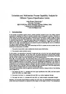
Figure 1 - Two types of surface tolerance profiles

With

Figure 1 shows two examples of a typical profile of surface tolerances. The first one does not refer to a datum frame (TYP 1) but the second one does (TYP 2). Please refer to the ASME Y14.5(.1)M-1994 standard for a more detailed explanation of these tolerances. The theoretical shape of a part is defined by nominal features characterized by basic dimensions or by mathematical models contained in the CAD file. To allow for faster control of a part, industrial habits propose defining a group of strategically chosen key characteristics (KCs). Generally, the profile of the part is controlled by a finite number of coordinate points NOMINAL Xi . The subscript ()i represents the rank of the control point ( 1  i  n ).The number n can be interpreted as a measure of the geometric complexity of the profile of the part. In fact, on a geometrically simple part, it is common to use a small number of measuring points, compared to a more complex geometry where n has to be a lot higher (Figure 2). Each X i represents a measure of the real shape of the controlled surface. This measure can be interpreted as NOMINAL the addition of the nominal value X i and  i . This error regroups the variations induced by fabrication and assembly processes, and also from measurement uncertainties (Chase, Magleby, and Glancy 1997). Xi  Xi

nominale

 i

(3)

f ( i )  N (  X i  X iNOMINAL ; X i )

B

(1)

NOMINAL

Xi

considered

i

and

with

i

f ( i ) 

With

 (  i   )

2

i

1 2  

e

2 

2

(4)

i

i

     and    0 . The cumulative i

i

distribution function (CDF) of  i is : F ( i )  Pr( w   i ) 

1

 1  erf 2 

  i      2

i

i

   

(5)

2. CAPABILITY OF THE PROFILE OF SURFACE TOLERANCE WITH SIX DEGREES OF FREEDOM

Figure 3 illustrates an example of the profile of a surface tolerance without datum according to the Y14.5 standard. The tolerance zone has six degrees of freedom and can be positioned anywhere and orientated anyhow inside the dimensional envelope. In this case, the tolerance guarantees that every single measured point will be inside two imaginary parallel profiles, spaced from each other by the value indicated in the tolerance box without any positioning or orienting constraint. ... N

M M

It is from this error that both types of profile of surface tolerances will be calculated from, as per the Y14.5

constant

    X , the PDF of the error  i is then defined as:

n

Figure 2 - Number of measuring points versus the geometrical complexity of the part

a

A

C

N

B

Figure 3 - Profile of surface tolerance without datum

 Referring to Y14.5.1, for each nominal point PN of the

 C pk are shown in Figure 5. In this case, the mean of the

profile (see Figure 4), there is a corresponding normal vector Nˆ to the surface. The value of the tolerance zone is equal to the sum of two intermediary tolerances t  et t  . They represent the allowed deviations

error has no influence on the value of the profile of surface tolerance of TYP 1.

Tol99.865%

following the positive and negative directions of the  normal vector Nˆ at a certain point PN . The actual  surface is defined by a defined group of points PS ,  representing points PN from the nominal profile to which an error  i is added. A profile is acceptable if, and only if, every actual point is inside the indicated    ( PN  t  )  PS  ( PN  t  ) where tolerance zone:   PS  PN   i . The profile of a surface tolerance zone

 Figure 5 - z pst versus C pk and the complexity n

without datum ( z pst  0 ) is equal to the difference of the normal vectors  i

max

et  i

min

of a profile, giving:

z pst  max( i )  min( i ) i 1, n

Table 1 and Table 2 present the results of x50% and (6)

i 1, n

x99.865%

for each case of  

for most of the i

complexities (5 ≤ n ≤ 500). Table 1 : x50% versus the complexity n and  

i

For the statistical development of the profile of surface tolerance with 6 degrees of freedom see Proof 1. Due to the complexity of the mathematical models developed, a MCS based on Eq.(6) will be used to be able to illustrate the value of z pst versus the geometric complexity of a part. The sample size was chosen based on two criteria: accuracy of the results and the elapsed time to complete the simulation. The resulting statistical distribution is unilateral and according to (Bothe 2006), the following equation must be used to take in account the capability of the process:    USL  x50% (7) Ppk , C pk    x99.865%  x50%

0.25 0.50 0.75 1.00 1.25 1.50 1.75 2.00 2.25 2.50

5 0.57 1.15 1.72 2.30 2.88 3.44 4.03 4.59 5.18 5.76

10 0.77 1.54 2.32 3.10 3.87 4.64 5.42 6.18 6.96 7.72

15 0.87 1.75 2.63 3.51 4.37 5.24 6.12 7.00 7.89 8.75

20 0.94 1.88 2.82 3.77 4.71 5.65 6.60 7.53 8.48 9.41

25 0.99 1.98 2.98 3.96 4.95 5.96 6.94 7.93 8.93 9.92

50 1.13 2.27 3.41 4.54 5.68 6.80 7.94 9.08 10.21 11.34

100 1.26 2.53 3.80 5.06 6.33 7.58 8.86 10.11 11.38 12.65

Table 2 : x99.865% versus the complexity n and  

500 1.53 3.06 4.59 6.12 7.64 9.18 10.70 12.21 13.77 15.27

i

x99.865%

 values values

Figure 4 - Representation of  i normal vector

 values values

x50%

0.25 0.50 0.75 1.00 1.25 1.50 1.75 2.00 2.25 2.50

5 1.24 2.52 3.78 5.01 6.29 7.57 8.76 10.03 11.30 12.59

10 1.34 2.67 4.01 5.38 6.73 8.03 9.41 10.69 12.06 13.40

15 1.40 2.81 4.19 5.62 6.98 8.38 9.79 11.15 12.60 13.95

20 1.44 2.88 4.31 5.79 7.20 8.64 10.11 11.50 12.95 14.39

25 1.48 2.95 4.41 5.88 7.34 8.79 10.29 11.78 13.21 14.77

50 1.57 3.15 4.72 6.26 7.84 9.41 11.02 12.57 14.08 15.72

100 1.67 3.33 5.01 6.67 8.31 9.96 11.68 13.36 14.98 16.64

500 1.87 3.74 5.62 7.52 9.37 11.25 13.13 14.97 16.86 18.75

A Weibull distribution is used to model z pst ( i ) distribution, so the formula to find a % percentile is: 1

   %  x%     ln  1     100  

(8)

Results for the profile of surface tolerance without datum for  i  N (0;1) , 5 ≤ n ≤ 50, and for different

3. CAPABILITY OF THE PROFILE OF A SURFACE TOLERANCE WITHOUT ANY DEGREES OF FREEDOM

Figure 6 shows an example of the profile of a surface tolerance with datum as per Y14.5 standard. In this case, the tolerance zone has to be controlled from the established datum reference frame.

M

Table 4. Values of x99.865% in relation to n and  / 

... A B C N

M

x 99 .865 % N

A

C

 

B

Figure 6 - Profile of surface with datum tolerance The tolerance zone is controlled from the datum reference frame with basic dimensions and is equal to the value indicated in the tolerance box. If not specified, it is equally spaced on each side of the nominal profile of the part. Therefore, the profile of a surface tolerance zone with datum z pstd is equal to the maximum value of the absolute values of the error vectors  i , multiplied by two: z pstd  2 max(|  i |)

(9)

i 1, n

For the statistical development of the profile of surface tolerance with 6 degrees of freedom, see Proof 2. The final analytical expression for z pstd is:

fz

pstd

2  

0.5  n

n



  e 

z pstd 2  4  2 4 2

 z  erf    2

pstd

( z pstd  2  )  ( z pstd 22  ) 2  e 8  e 8   2

 2 2

 z   erf    2

pstd

 2 2

2

   

n 1

  (10)  

Again, the Eq.(7) is used to define the capability of the process. Because both  and   have an influence on the i

0.00 0.50 1.00 1.50 2.00 2.50

5 7.29 7.93 8.92 9.92 10.93 11.92

10 7.64 8.29 9.29 10.29 11.29 12.29

15 7.84 8.50 9.50 10.50 11.50 12.50



Complexity n 20 25 7.97 8.08 8.64 8.75 9.64 9.74 10.64 10.74 11.64 11.75 12.64 12.74

50 8.40 9.08 10.08 11.08 12.08 13.07

100 8.71 9.40 10.40 11.40 12.40 13.40

500 9.40 10.10 11.10 12.10 13.10 14.10

4. CASE STUDY I

In this case study we will look at the assembly of a floorboard on a tubular stainless steel structure assembled by a welding process. The complexity of the stainless steel structure is estimated at n = 50. Glue is used to assemble the two parts and the specifications require a minimum thickness of 1 mm to provide enough retaining force. The thickness of the glue must be 1-10 mm . The company’s manufacturing department also added in its assembly process the use of 5 mm shims to ensure that the floorboard never makes direct contact with the stainless steel. In doing so, they want to avoid any damage to the floor by the welds. Before starting production, the manufacturing engineer wants to check if the company’s welding process is able to determine if the number of non-conform assemblies will be acceptable. From previous studies, the welding process error that includes withdraws, the jig’s error, and the inspection error, was statistically adjusted to a normal distribution with  welding  0.25 mm and

 welding  0.50 mm. The maximum profile of a surface tolerance without datum allowed for the structure is 3.50 mm to respect the minimum glue thickness and 4.5 mm to respect the maximum drying time. The lowest tolerance is used to verify the process capability.

i

value of z pstd , two charts were constructed from the above mathematical models to facilitate the calculation of the tolerance with Eq.(7). Table 3 and Table 4 present the results of x50% and

fl oorboard glue

 

x99.865% for different cases of  /  and n. structure

shims

Table 3. Values of x50% in relation to n and  /  x50%

 

0.00 0.50 1.00 1.50 2.00 2.50

5 3.04 3.40 4.27 5.26 6.26 7.26

10 3.67 4.09 5.01 6.00 7.00 8.00

15 4.01 4.46 5.39 6.39 7.39 8.39

Figure 7 – Floor structure with a complexity of n=50



Complexity n 20 25 4.24 4.42 4.71 4.90 5.65 5.85 6.65 6.84 7.65 7.84 8.65 8.84

50 4.93 5.45 6.41 7.41 8.41 9.41

100 5.41 5.96 6.93 7.93 8.83 9.93

500 6.40 7.00 7.99 8.99 9.99 10.99

From Table 1, Table 2, and Eq.(8) we find x50%  2.27 and x99.865%  3.15 which gives a capability index of C pk  1.40 . If we consider that the lowest C pk is 1.33

for a process to be acceptable, we can conclude that the welding process used to build the floor’s structure is capable.

5. CASE STUDY II

Two existing sub-modules have to be put together to form a new module. Again, the engineers want to verify if their welding processes are capable to produce the desired KC. Sub-module 1 complexity is set to n = 10 and sub-module 2 to n = 25. Here the KC is the gap between the right side of sub-module 1 and the left ends of sub-module 2 when they are put together in the main welding jig. This gap (KC) has to be within 0 mm and 4 mm to obtain the best quality for geometrical variations.

considering the geometrical complexity of the part and its process capabilities. The mathematical model based on order statistics and statistical tolerance analysis methods, allowed us to construct charts for each type of tolerance. Two case studies showed the usefulness of the developed models for designers.

Proof 1 From the order statistics theorem (Papoulis 1991), we can find the PDF formula for the minimum and the maximum of  i . This theorem says that the statistical distribution of a ranked variable yk is defined by: g k ( yk ) 

n! ( k  1)!( n  k ) !

F

k 1

[1  F ]

nk

f ( yk ) (12)

The maximum max(  i ) and the minimum min(  i ) values being the nth rank are obtained from eq.(12) with k = n and 1 respectively, which gives: f max ( i )  n[ F ( i )]

n 1

f ( i )

f min ( i )  n[1  F ( i )]

Figure 8 – New assembly modules Sub-module 1 welding process produces an error with

 welding  0.50 and  welding  0.25 and its nominal 1

1

n 1

f ( i )

(13)

Overlapping Figure 9, we can see the tendency of both functions max( i ) and min( i ) compared to the original function  i = N(0,1). The higher the geometric complexity of the profile, the bigger the difference between extremes values of  i .

width is 500 mm. The other sub-module’s welding process produces an error with  welding  0.25 and

0.8

 welding  0.50 and its nominal width is 498 mm. This

0.7

gives a nominal gap value of 2 mm. To verify the capability of the welding processes to respect the KC, we need to estimate each module’s profile of surface tolerance with reference to their respective positioned side in the main welding jig. Sub-module 1 datum is then its left side, and sub-module 2 its right side. With the help of Table 3, Table 4 and Eq.(7) and considering a minimum C pk of 1.33, the z pstd of

0.6

2

sub-module 1 is 3.18 mm and sub-module 2 is 5.01 mm. Assuming that each tolerance is equal to six standard deviations, if we perform statistical tolerance analysis, it gives a standard deviation of 0.99 for the gap. This means that you could get an interference of 1 mm instead of the minimum 0 mm gap, and a maximum gap of 5 mm. In conclusion, the welding processes are not capable to respect the KC.

6. CONCLUSION In this study, we developed a methodology to statistically estimate both types of profile tolerances according to the ASME Y14.5(.1)M-1994 standard,

0.5 0.4 0.3 0.2 0.1 0 -4

-2

0

2

4

Figure 9 - PDF’s of min(  i ) and max(  i ) If x and y are two independent random variables, the PDF of their sum is equal to the convolution of their PDFs. Then for z = x + y : 

fz ( z) 

 f ( z  y ) f ( y )dy x

y

(14)

0

In our case, from Eq. (6) we z pst  max( i )  min( i ) , and analogically :

have

f z  f z ( i )

f z ( z pstd ) 

pstz

f x  f max ( i )

pstd

(15)

f y  f min  ( i )   f min ( i )

Again, when y  ax  b :

 yb    a 

1

fx 

|a|

(16)

f min  ( y )  f min (  y ) .

We must substitute Eq.(13) into Eq.(16) to obtain the PDF of the profile of surface tolerance without datum. Due to the complexity of the model, a Mont-Carlo simulation based on eq. 6 has to be performed to study the behavior of z pst . Proof 2 From Eq.(9), we can estimate the following z pstd  2 max( i ) 2

x   i , then

(17)

z pstd  2 max( x ) .

2

According to the order statistics theorem, the PDF and CDF of x respectively are : f x ( x) 

Fx ( x ) 

1 2



2 x

(

e

x  ) 2

2

2

2   1  e  

x 2

  

(18)

  x    x     Erf    Erf    (19) 2  2   2  

1

In this case, the resulting statistical distribution is a  with one degree of freedom. Again, from Eq.(12), the PDF of max( x ) is: 2

f max ( x, n )  nFx If, y 

n 1

f x ( x)

(20)

max  x  , then: f y ( y )  2( y ) f max ( y )U ( y ) 2

(21)

The following expression is the analytical solution for f y ( y ) with y  0 : 2  20.5 n n    ( y22) f y ( y)     e    

(23)

REFERENCES

For our case, if a = -1, b = 0, then:

Assuming that

|2|

 z pstd    2 

fy 

The finally analytical expression provides the solution for the PDF of z pstd  0 is given in Eq.(9).

Before applying the convolution, we must find f min  .

f y ( y) 

1

2 y  2 1  e  

  y   y      erf    erf    2   2   

(22) And from Eq.(22), and with

z pstd  2 y , the PDF of

the profile of surface tolerance with datum becomes :

n 1

   

[1] Ameta, G., J. K. Davidson, J. J. Shah, “Tolerance-maps applied to a point-line cluster of features”. J of Mechanical Design, Trans. of the ASME Vol. 129, No. 8:pp782-792, 2007. [2] ASME Y14.5(.1)M – 1994, “Dimensioning and tolerancing”, American Society for Mechanical Engineering, 2002. [3] Bothe, D. R., “Assessing capability for hole location”, Quality Engineering, Vol. 18, No. 3, pp325-331, 2006 [4] Chase, K. W., “Minimum-cost tolerance allocation”, ADCATS Report No. 99-4&5, Brigham Young University, 1999 [5] Chase, K. W., P. M. Spencer, C. C. Glancy, “A comprehensive system for computer-aided tolerance analysis of 2-D and 3-D mechanical assemblies”. Proc 5th Int Conf on Computer-Aided tolerancing, Toronto, Canada, 1997. [6] Chen, Yong, Y. Ding, J. in, D. Ceglarek, “Integration of process-oriented tolerancing and maintenance planning in design of multi-station manufacturing processes”. IEEE Trans on Automation Science and Engineering, Vol. 3, No.4, pp440-453, 2006 [7] Cox, N. D, “How to perform statistical tolerance analysis”, The ASQC Basic References in Quality Control: Statistical Techniques 11, 1986. [8] Huang, W. J. Lin, M. Bezdecny, Z Kong, D. Ceglarek, “Stream-of-variation modeling - Part I &II”, J of Manufacturing Science and Engineering, Vol. 129, No. 4, pp821-842, 2007 [9] ISO 21747, “Process performance and capability statistics for measured quality characteristics”, Int Standard Organization, 2006. [10] Montgomery, D. C., G. C. Runger, “Applied statistics and probability for engineers”, 4th ed John Wiley & Sons, 2007. [11] Papoulis, A., “Probability, random variables, and stochastic processes”, 3rd ed, McGraw-Hill, 1991. [12] Xiong, C., Y. Rong, R. P. Koganti, M. F. Zaluzec, N. Wang, “Geometric variation prediction in automotive assembling”, Assembly Automation, Vol. 22, No. 3, pp260-269, 2002. [13] Zhang, Yu, Musheng Yang, and Yanxin Zhang, “Concurrent Design for Process Quality, Statistical Tolerance, and SPC”, Com in Statistics - Theory and Methods , Vol. 35, No. 10, pp1869-1882, 2006.