Exploiting Time-Malleability in Cloud-based Batch Processing Systems. Luo Mai. Imperial College London. Evangelia Kalyvianaki. City University London.
Exploiting Time-Malleability in Cloud-based Batch Processing Systems Luo Mai Imperial College London
Evangelia Kalyvianaki City University London
Abstract Existing cloud provisioning schemes allocate resources to batch processing systems at deployment time and only change this allocation at run-time due to unexpected events such as server failures. We observe that MapReduce-like jobs are timemalleable, i.e., at runtime it is possible to dynamically vary the number of resources allocated to a job and, hence, its completion time. In this paper, we propose a novel approach based on time-malleability to opportunistically update job resources in order to increase overall utilization and revenue. To set the right incentives for both providers and tenants, we introduce a novel pricing model that charges tenants according to job completion times. Using this model, we formulate an optimization problem for revenue maximization. Preliminary results show that compared to today’s practices our solution can increase revenue by up to 69.7% and can accept up to 57% more jobs.
1
Introduction
MapReduce and its derivatives such as Dryad and Spark are the de-facto standard to execute batch jobs in a cloud environment. They support a simple programming model that limits the dependencies among their sub-tasks, leading to a flexible mapping between tasks and resources. This allows jobs to scale out to run on an arbitrarily large number of servers, without requiring any additional effort from programmers. The constrained programming model and fixed dependencies among tasks also simplify the estimation of the job execution time and several estimation models, which take into account job characteristics, input data size, and the resources allocated, have recently appeared in literature [5–7, 10, 11].
Paolo Costa Microsoft Research
Several systems build upon this predictability at deployment time to derive the number of resources needed to meet user specified deadlines [6, 7, 11]. Small allocation adjustments can be made at runtime in order to cope with unexpected and not-so-common events such as server failures [5]. A major drawback of these approaches, however, is that the provider is bound to a fixed allocation plan. This is at odds with the elastic nature of cloud where available resources fluctuate over time. In contrast, we propose an approach that deliberately varies the amount of resources allocated to jobs over time in order to control their completion time and increase cloud utilization. The intuition is that if spare resources are available, they should be allocated to running jobs to reduce their completion time. However, if new jobs are submitted, these resources should be claimed back to accommodate the new jobs. Our approach builds upon the observation that most (if not all) MapReduce-like jobs are timemalleable, i.e., it is possible to change their resource allocation at runtime, without affecting the correctness of the results [2, 7]. A key challenge of our approach is that under the current, pay-as-you-go, pricing model, there is no incentive for the provider to reduce execution time. Even with the recently proposed deadlinebased models, e.g., [7, 8], users can only specify a single desired completion time. To address these shortcomings, we combine our solution with a novel pricing model in which the later a job is completed, the lower users pay. However, to avoid unbounded completion time, users also specify the longest acceptable deadline of their jobs. Dually, they also indicate the maximum price they are willing to pay. We believe that this model is advantageous to both
A
A
A
A
B
A
A
A
B
B
B
B
B
B
B
1
2
3
4
5
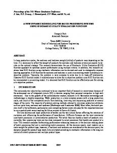
malleability, it is possible to dynamically change the allocation plan, exploiting the loose deadline of B to accommodate C and potentially increase its revenue. Figure 1(b) shows such a reconfiguration that leads to feasible allocation plans for jobs B and C. Besides meeting the deadlines of current jobs, the provider also aims at maximizing its revenue. Therefore, while reallocating resources, it must ensure that the total revenue does not decrease as a consequence of accepting a new job and delaying an already running one. The next section presents our solution to this problem.
B resource unit
6
7
time interval
(a) Allocation plan for jobs A and B A
A
A
A
B
B
B
A
A
A
C
C
B
B
B
B
C
C
C
B
B
1
2
3
4
5
6
7
resource unit
time interval
(b) Runtime reallocation for new job C
Figure 1: Example of dynamic resource allocation
3
Allocation for time-malleable jobs
users and the provider. It provides great incentives users to define a long deadline in the exchange of a reduced price. At the same time, this model also benefits the provider to devise flexible planning decisions among all jobs. In this paper, we take a first step in this direction by formulating the allocation problem as a mixed integer program to maximize provider’s revenue (Section 3.2). Our work relies on existing work to derive the initial resource requirements for jobs at deployment and we extend our formulation to consider related errors at runtime (Section 3.3). Simulation results show that our approach significantly improves both provider revenue and jobs acceptance ratio. (Section 4).
In this section, we formulate the problem of cloud revenue maximization. We first present a basic formulation, followed by an adjustment that takes into account errors in the estimations of jobs resource requirements. Overall a new job is accepted if and only if the solution to the maximization problem provides a feasible allocation plan with an estimated revenue higher than the revenue coming from the current allocation without the new job. A user with a new job j communicates to the provider the longest acceptable deadline d j and the number of resource units required r j . The user and the provider also agree upon a pricing function described below.
2
A pricing function P(t) describes the relationship between the job completion time t and the corresponding price to be paid to the provider. To build such a function, the user indicates the longest acceptable deadline (hereafter referred to as the deadline) of her job d. The user and the provider also agree upon a maximum affordable price pmax paid if the job finishes at an earliest possible completion time s. A pricing function that captures the fact that a job should cost less for longer completion times is: if t < s pmax f (t) if s ≤ t ≤ d P(t) = 0 if t > d.
3.1
Overview
We illustrate our approach by means of the example in Figure 1. We assume a cloud data center with three resource units (e.g., a VM or a MapReduce slot) at any given time. Consider two jobs, A and B, with the following requirements: (rA = 7, dA = 6) and (rB = 9, dB = 7), where r j denotes the total resource units for job j and d j shows the completion time deadline of j counting from its sumbission time. We assume an initial feasible allocation plan as depicted in Figure 1(a); an allocation plan shows the number of units allocated to a job at any given time. A plan is feasible when the total allocation of resource units per interval does not exceed the cloud capacity. Let us now suppose that a new job C is submitted at time t = 2 with the requirements (rC = 5, dC = 3). Under today’s rigid allocation scheme, job C could not be accommodated, since by the time B completes at t = 6 and resources become free, C’s deadline has already expired. However, by exploiting job time-
Pricing function on completion time
Figure 2 provides an example P(t). In the range where (s ≤ t ≤ d), the price f (t) of a job completion time t should be monotonically decreasing to t and its values never exceed pmax . Figure 2 shows a convex function; but different shapes can be considered as well. Note that if (t > d) then the job fails to meet its deadline and no payment is issued. 2
cost
time job
P max
actual cost
2
1
job 1
(x12 , y12 )
job 2
(x21 , y21 ) (x22 , y22 )
...
k
...
...
(x2k , y2k )
...
job 2 finishes at time k y2k = 1
time s
t actual job completion time
d deadline
job N
Figure 2: Example of a pricing function Pj of job j.
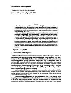
Consider N − 1 jobs running under certain allocation plans and a new job arriving. Our goal is to find a feasible allocation for the new job that maximizes the total revenue for all N jobs over time. To find a set of feasible allocation plans we formulate the mixed integer programming (MIP) problem with the objective (1) subject to constraints (2)- (6). We solve the maximization problem for a duration of T = arg max j d j intervals to include the longest deadline among all N jobs. We use t to index intervals for the next T intervals starting from the current one pointed by t = 1, i.e., t ∈ {1, . . . , T }. We ensure that the solution includes feasible plans via the constraints explained below. We also use Figure 3 to illustrate key points of the constraints.
j
xj2 K
∀ j,
(2)
∀ j,
(3)
∀t,
(4) (5)
3.3
(6)
Our model uses an estimate of the number of resource units required by a job. Recent work on offline profiling and analytic performance models derive the resource units required for MapReduce jobs e.g., [5, 7, 10, 11]. Further, some workloads exhibit a large fraction of recurring jobs. For example, in Bing’s production clusters recurring jobs account for 40.32% of the total [1]. This allows to improve the prediction by taking into account prior executions. Nevertheless, despite the accuracy of these initial estimations, it is still possible that discrepancies arise during job execution, e.g., due to stragglers [3, 12]. Therefore, we extend our basic formulation to accommodate for estimation errors. We insert a random parameter e j , referred to as the
N
(1)
x,y,p
dj
0
x2i = r2
resource units per job j at interval i. The number of dj resource units before the deadline, i.e., ∑i=1 x ji , must be equal to r0j ; where r0j ≤ r j denotes the remaining resource units needed to allocate for job j given that j might be an existing running job and has already used some of its resource units. The sum of allocations across jobs per interval must not exceed the total cloud capacity denoted by K and shown by (4). Furthermore, the resource allocation x ji itself cannot exceed the total capacity of the cloud and is shown by (5). Finally, constraint (6) denotes the payment of a job given its completion time and where t˜j denotes the previous running time of job j. This payment is bounded by function Pj (t). The problem to find the optimal solution for a MIP formulation has shown to be NP-complete. Therefore, we use the CPLEX state-of-the-art optimization solver [13] to find approximated solutions within short times.
maximize ∑ j=1 p j
∑i=1 y ji = 1 d ∑i=1 x ji = r0j N ∑ j=1 x jt ≤ K
i=1
Figure 3: Example illustration of the constraints and the decision variables x and y.
Cloud revenue maximization
subject to
(x2T , y2T )
Xd2
(xN 2 , yN 2 ) XN
j=1
3.2
T = d2
T
0 ≤ x jt ≤ K × ∑i=t y ji ∀ j,t, � � dj p j ≤ Pj t˜j + ∑i=1 i × y ji ∀ j,
y ji ∈ BN×T , x ji ∈ NN×T , p j ∈ R+ , (7) j ∈ {1, . . . , N}, t ∈ {1, . . . , T }. (8)
Deadline feasibility constraint. All jobs should finish before their deadlines shown by (2) where the binary variable y ji ∈ BN×T is assigned to 1 if job j completes at time i, otherwise is set to 0, also shown in Figure 3. For every job j there should be only one y ji = 1 at a time before its deadline d j . Resource feasibility constraints. All jobs should be given resource units according to their requirements shown by (3) and exemplified in Figure 3. The decision variable x ji ∈ NN×T denotes the allocation of 3
Discrepancies in resource estimation
of the pricing function in Figure 2 are randomly choj j sen and s j ∈ [dmin , 5 · dmin ] and d j ∈ [s j , 3 · s j ]. Note that this setup implies that some jobs may have no flexibility at all, i.e., s j = d j . For simplicity we consider a linear pricing function Pj . We also experimented with different function shapes and different ranges for s j and d j , observing similar trends to the results reported below. We simulate job requests arriving over time for a total duration of 10,000 seconds. We assume Poisson job arrivals with a mean arrival rate λ varying between 0.12 and 0.26 jobs/s (resp. 0.30 and 0.65 jobs/s for the Google-inspired workload). These values yield a data center utilization between 60% and 100% when we allocate resources. Baselines. We compare our approach against three baselines, representative of common techniques used in today’s systems. E ARLY: a fixed set of resources is reserved for a job to meet its most demanding deadline s j . This closely resembles the existing approach in deadline-based systems where a single deadline is considered. L ATE: a fixed set of resources is reserved for a job to meet its deadline d j ; E DF: this baseline implements an earliest deadline first (EDF) approach where we allow runtime modifications in jobs allocation plans; we consider the deadline d j . CPLEX execution time. We run our experiments on a server with 16 Intel Xeon E5-2690 cores and 32 GB of RAM. We set the upper bound of the CPLEX execution time per job to 100 s and the error rate to 1%. Across all runs1 , the median CPLEX execution time is 2 s and the 95th percentile is 6 s. Since our algorithm needs to be run only when a job is submitted, the overhead introduced is negligible.
job size estimation error, into constraint (3) to introduce the job execution variability in planning, i.e., rj e j . For example, when e j ∈ (0, 1) then the size of the job is underestimated (resp. overestimated if e j > 1). Hence, constraint (3) can�be transformed � into a probd
r0
j ability constraint: Prob j ∑i=1 x ji = e jj ≥ 1−α, ∀ j. This rewritten constraint ensures that, with a (1−a) probability guarantee, the accumulated number of resource units allocated to a job before its deadline equals its remaining job size considering any estimation errors. Using a probability constraint makes the program stochastic and cannot be solved by standard solvers like CPLEX. To calculate the solution to it, we transform it into a deterministic equivalent by assuming that e j is subject to a normal distribution, i.e., e j ∼ N(µ j , σ 2j ). Due to space limitations we omit the details of the transformation. At the end, the transformed formulation can be solved with CPLEX.
4
Preliminary Results
To quantify the benefits achieved by the formulation approach outlined in Section 3 (hereafter, referred to as G EAR B OX), we use a discrete event simulator and CPLEX to solve the maximization problems. While preliminary, our results indicate that by allowing users to specify long deadlines and by exploiting time-malleability our approach increases both provider revenue and acceptance ratio.
4.1
Setup
Given the unavailability of a reference workload that would fit our pricing model, we adopt a synthetic workload. While admittedly simplistic, we believe that this workload is a good approximation of what a real workload might be. We assume a cloud with a total capacity of K = 1, 000 resource units. We denote r j to be the initial r j number of units required by job j; dmin = Kj is the shortest completion time possible when all cloud resources are assigned to j. We consider two different scenarios. In the former (Figure 4), we assign the initial resource requirements r j of job j to be a randomly chosen integer between 2,500 and 7,500 resource units. This ensures that all jobs take at least j more than two units of time to complete (i.e., dmin >2 for all jobs). In the latter scenario (Figure 5), we set r j = 50 · (1 + b), where b is randomly selected using a half-normal distribution with a mean of 0 and standard deviation of 50 modeled after the analysis from Google cluster traces [9]. The parameters s j and d j
4.2
Basic formulation results
We begin our analysis by considering the case with no estimation errors. Figure 4(a) shows the percentage of jobs accepted by each method. We observe that the dynamic allocation plans (G EAR B OX and E DF) accept significantly more jobs than the static ones (E ARLY and L ATE). The reason is that, by being unable to reallocate resources as new jobs come in, or existing jobs terminate, the performance of static allocation plans is drastically reduced. This highlights the problem with today’s setup and motivates our effort to explore alternative solutions. The second metric used in our evaluation is the 1 We
average the results across 5 runs and the standard deviation for all experiments in this section is within 3%.
4
EARLY LATE
Revenue (relative to EARLY)
Accepted jobs (%)
100 80 60 40 20 0
EARLY LATE
GearBox EDF 1.8
GearBox-97.5 GearBox-90 Revenue (relative to EARLY)
GearBox EDF
1.6 1.4 1.2 1 0.8 0.6
0.1 0.12 0.14 0.16 0.18 0.2 0.22 0.24 0.26
1.8 1.6 1.4 1.2 1
0.1 0.12 0.14 0.16 0.18 0.2 0.22 0.24 0.26
Inter-arrival rate (λ)
0.1 0.12 0.14 0.16 0.18 0.2 0.22 0.24 0.26
Inter-arrival rate (λ)
(a) Job acceptance ratio
EDF GearBox
(b) Total revenue
Inter-arrival rate (λ)
(c) Total revenue with estimation errors
Figure 4: Simulation results with the job sizes generated using a uniform distribution EARLY LATE
Revenue (relative to EARLY)
Accepted jobs (%)
100 80 60 40 20 0
EARLY LATE
GearBox EDF 1.8 1.6 1.4 1.2 1 0.8 0.6 0.4
EDF GearBox
1.8 1.6 1.4 1.2 1
0.25 0.3 0.35 0.4 0.45 0.5 0.55 0.6 0.65
0.25 0.3 0.35 0.4 0.45 0.5 0.55 0.6 0.65
Inter-arrival rate (λ)
Inter-arrival rate (λ)
(a) Job acceptance ratio
GearBox-97.5 GearBox-90 Revenue (relative to EARLY)
GearBox EDF
(b) Total revenue
0.25 0.3 0.35 0.4 0.45 0.5 0.55 0.6 0.65 Inter-arrival rate (λ)
(c) Total revenue with estimation errors
Figure 5: Simulation results with the job sizes generated using a half-normal distribution [9] total revenue, shown in Figure 4(b), normalized against E ARLY. G EAR B OX achieves much higher revenue than E ARLY (between 53.7% and 69.7%) and L ATE (between 170% and 205%). This is because of G EAR B OX’s ability to dynamically reassign resources and, hence, accept more jobs. Interestingly, G EAR B OX also outperforms E DF (between 5.6% and 17.5% higher revenue), although their fraction of accepted jobs is close. The reason is that G EAR B OX admits a new job only if this increases the total revenue. This means that in some cases, even if there would be enough idle resources to accept a job, G EAR B OX can still decide to reject it, if this is not cost-effective. In contrast, if resources are available, E DF always accepts a new job, although this might be detrimental in the long term. This shows the importance of considering the total revenue as a first-class citizen in the admission control. Similar trends are also observed when using the Google-inspired workload as shown in Figure 5.
utilizes resources as soon as they become available and, hence, it is more prepared to accommodate future bursts of jobs. Furthermore, and in contrast to E ARLY, it also has the ability to reclaim resources back from running jobs as appropriate for new ones. Interestingly, at low load (λ = 0.12), the median job completion time increase (relative to s j ) is less than 1% (95th percentile is 46%). At high load (λ = 0.26), instead, the median is 26% (95th percentile is 177%). This indicates that G EAR B OX exploits timemalleability only for a few jobs, while for the vast majority of them, it strives to minimize the completion times. This is a consequence of the incentives set by our pricing model. The provider has a strong incentive to finish the job as soon as possible. At the same time the provider can delay a few jobs if this increases the overall revenue.
4.3
Estimation errors
We now consider the impact of estimation errors on our base solution, G EAR B OX, and show how the extension detailed in Section 3.3 can mitigate these. We refer to our extended solution as G EAR B OX-p, where p is the probability in the transformed constraint. We assume that the estimation error e j for a job j follows the normal distribution N(1, 0.1). This is consistent with the results presented in [6,7]. We also experiment with other values of standard deviation
We also experimented with a flat pricing function, obtaining a factor of 1.8x improvement in the revenue of G EAR B OX over E ARLY (resp. 1.1x over E DF). This shows that even when there is no additional premium for the provider to complete jobs early, it can still increase its revenue by exploiting their malleability. This is because G EAR B OX fully 5
σ ∈ [0.05, 0.15], obtaining similar results. Figure 4(c) and 5(c) show the revenue for different job inter-arrival rates λ in the two workloads considered. G EAR B OX-97.5 and G EAR B OX-90 achieve higher revenue than both E DF and G EAR B OX. In this scenario, E DF outperforms G EAR B OX because as it recomputes the deadlines at runtime, it naturally shifts resources to jobs that are close to deadlines, thus implicitly accounting for estimation errors. However, the G EAR B OX-p solutions achieve the best performance because they account for estimation errors in their allocation plans. This is also reflected in the fraction of accepted jobs that miss the deadline. While E DF and G EAR B OX exhibit a miss ratio of 6.05% and 13.75% respectively, G EAR B OX-90 achieves a miss ratio of 0.7% (respectively 0.07% for G EAR B OX-97.5).
5
6
Conclusions
Current batch processing systems support fixed allocation plans, in which the resources allocated to a job are never changed (unless in cases of unexpected events such as failures or stragglers). Rather, we argue that the time-malleability property of batch jobs should be exploited to opportunistically vary the allocation plans at runtime. Our approach allows users to specify the longest acceptable deadline for their jobs along with the maximum price they are willing to pay. Providers then use this information to dynamically allocate resources to jobs in order to improve utilization and revenue. Preliminary results show that our approach can significantly increase revenue and acceptance rate, by only marginally affecting job execution time. Acknowledgements. The authors wish to thank Wolfram Wiesemann for his helpful comments and suggestions, and Bolun Dong, James Simpson, and Jiawei Yu for their help on building a preliminary prototype of our system. Luo Mai is a recipient of the Google Europe Fellowship in Cloud Computing, and this research is supported in part by this Google Fellowship.
Discussion
We are implementing our approach in the Apache Hadoop framework. Our prototype currently supports dynamic reallocation in the map phase. Since map tasks are short, independent and run in multiple waves, we can vary the number of resources between each wave. Reduce tasks are more complex as they are typically long-running and they run in a single wave. To support dynamic reallocation in the reduce phase, we are currently integrating our prototype with the Sailfish project [2, 14], which supports suspend and resume of reduce tasks. The current version of the model makes some simplifying assumptions. In particular, we assume perfect scalability and ignore data dependencies. For a real deployment, our model needs be extended to include constraints such as job barriers, which can reduce parallelism, and data locality, which can have an impact on the total running time. Addressing these limitations as well as including network constraints (possibly leveraging our prior work [4, 7]) is part of our current research agenda. We also intend to explore more advanced pricing functions. In the results presented in the previous section, we assume static pricing, i.e., the shape and values of the function depend only on the job type and size. We are currently investigating the benefits of using dynamic pricing functions similar to the Amazon spot instances model [15], in which prices changes based on the current utilization. We believe that combining dynamic pricing with job malleability would allow to further increase utilization and revenue while providing more flexibility to tenants.
References [1] AGARWAL , S., K ANDULA , S., B RUNO , N., W U , M.-C., S TO ICA , I., AND Z HOU , J. Re-Optimizing Data-Parallel Computing. In NSDI (2012). [2] A NANTHANARAYANAN , G., D OUGLAS , C., R AMAKRISHNAN , R., R AO , S., AND S TOICA , I. True Elasticity in Multi-Tenant Data-Intensive Compute Clusters. In ACM SoCC (2012). [3] A NANTHANARAYANAN , G., K ANDULA , S., G REENBERG , A., S TOICA , I., L U , Y., S AHA , B., AND H ARRIS , E. Reining in the outliers in map-reduce clusters using Mantri. In OSDI (2010). [4] BALLANI , H., C OSTA , P., K ARAGIANNIS , T., AND ROWSTRON , A. Towards Predictable Datacenter Networks. In SIGCOMM (2011). [5] F ERGUSON , A., B ODIK , P., K ANDULA , S., B OUTIN , E., AND F ONSECA , R. Jockey: Guaranteed Job Latency in Data Parallel Clusters. In EuroSys (2012). [6] H ERODOTOU , H., D ONG , F., AND BABU , S. No One (Cluster) Size Fits All: Automatic Cluster Sizing for Data-intensive Analytics. In ACM SoCC (2011). [7] JALAPARTI , V., BALLANI , H., C OSTA , P., K ARAGIANNIS , T., AND ROWSTRON , A. Bridging the Tenant-Provider Gap in Cloud Services. In ACM SoCC (2012). [8] L UCIER , B., M ENACHE , I., NAOR , J., AND YANIV, J. Efficient Online Scheduling for Deadline-Sensitive Batch Computing. In SPAA (2013). [9] S CHWARZKOPF, M., KONWINSKI , A., A BD -E L -M ALEK , M., AND W ILKES , J. Omega: flexible, scalable schedulers for large compute cluster. In Eurosys (2013). [10] V ERMA , A., C HERKASOVA , L., AND C AMPBELL , R. H. ARIA: Automatic Resource Inference and Allocation for MapReduce Environments. In ACM ICAC (2011). [11] W IEDER , A., B HATOTIA , P., P OST, A., AND RODRIGUES , R. Orchestrating the Deployment of Computations in the Cloud with Conductor. In NSDI (2012). [12] Z AHARIA , M., KONWINSKI , A., J OSEPH , A. D., K ATZ , R., AND S TOICA , I. Improving MapReduce performance in heterogeneous environments. In OSDI (2008). [13] IBM, ILOG CPLEX. http://www.ibm.com. [14] Sailfish Project. http://code.google.com/p/sailfish/. [15] Amazon EC2 Spot Instances. http://aws.amazon.com/ec2/ spot-instances/.
6