Exploiting Wireless Channel State Information for Throughput Maximization V. Tsibonis, L. Georgiadis, L. Tassiulas
Abstract— We consider the problem of scheduling packets over a number of channels with time varying connectivity. Policies proposed for this problem either stabilize the system when the arrival rates are within the stability region, or optimize an objective function under the assumption that all channel queues are saturated. We address the realistic situation where it is not known apriori whether the channel queues are saturated or not, and provide a scheduling policy that maximizes the weighted sum of channel throughputs. We employ a burstiness-constrained channel model that allows us to dispense of statistical assumptions and simplifies the proofs. Index Terms— Scheduling, Deterministic network calculus, QoS in wireless networks.
I. I NTRODUCTION The primary motivation of this work is the problem of scheduling the transmissions of multiple data flows sharing the same wireless channel. The relative delay tolerance of data applications, together with the bursty traffic characteristics, opens up the potential for scheduling transmissions so as to optimize throughput. Given the above considerations, we examine a time-slotted parallel queue system with a single server. The condition of the associated channel of every queue varies with time between “on” and “off” states. In every time slot only one packet can be transmitted from a given queue, if the associated channel is in the “on” state and the queue is non empty. The main result of this paper is the design of a scheduling policy that allocates the server to the queues in such a way that the weighted sum of channel throughputs is maximal. A related approach along these lines is proposed in [4], where the authors identify optimality properties for scheduling downlink transmissions to data users, in CDMA networks. For arbitrary-topology networks, the problem of admission control and rate allocation to the users so that certain qualityof-service requirements are met, is investigated. A mathematical programming formulation is obtained for determining the optimal transmission schedule. The effect of wireless channels on the performance of transmission protocols such as TCP is examined through simulations in [5]. The authors conclude that channel-state scheduling can lead to significant improvement in channel utilization. The problem of scheduling wireless channels with time varying connectivity has been addressed in the past in several V. Tsibonis and L. Georgiadis are with Aristotle University of Thessaloniki, Thessaloniki, GREECE. e-mails:
[email protected],
[email protected] L. Tassiulas is with the University of Thessaly, Greece and University of Maryland, College Park. e-mail:
[email protected]
0-7803-7753-2/03/$17.00 (C) 2003 IEEE
different contexts. In [12], optimal scheduling for a wireless system consisting of multiple queues and a single server is studied. The arrival processes to the queues are assumed i.i.d Bernoulli. The wireless channels can be in the “on” or in the “off” state according to i.i.d Bernoulli processes. The authors derived the system stability region; moreover, they showed that the policy that among the queues whose channel is “on” serves the one with the longest queue, stabilizes the system whenever the arrival rates are within the stability region. In [13], Tassiulas considered a system that generalizes the one in [12] in the following aspects. First, a network with arbitrary topology is considered. Second, the topology is represented by a hidden Markov model instead of an independent and identically distributed (i.i.d) process. Third, anticipative scheduling policies are taken into consideration. Fourth, multiple link transmission rates are considered. In that context, after the characterization of the region of achievable throughputs, a transmission scheduling policy is proposed, that achieves all throughput vectors achievable by any anticipative policy. The problem of scheduling transmissions over a wireless channel with time-varying transmission rates is considered in [11], [6], [9] and [8]. The problem of providing a scheduling policy that stabilizes the system whenever the arrival-rate vector lies within the stability region is dealt in [11] and in [8]. In [11], a finite set of channel states is assumed and every channel can be in one of these states. With each state there is an associated data rate, representing the rate at which the queue is served if selected for transmission. The arrival processes to the queues are assumed mutually independent, ergodic, Markov chains with countable state space. Under these assumptions it was shown that the scheduling policy, called the exponential rule, makes the queues stable if there exists any policy that can do so. In [8], the authors consider the problem of power and server allocation in a multi-beam satellite downlink which transmits data to different ground locations over time varying channels. The authors establish the stability region of the system and develop a power allocation policy, which stabilizes the system whenever the system is stabilizable and when the arrival and channel state processes are i.i.d. In [9] and [6] the problem of developing a scheduling policy for efficient channel utilization is considered for the case that all the queues are unstable. In [9] the state of a channel is modeled by a stochastic process, which represents the level of performance of the given channel. A scheduling policy is provided which maximizes the average system performance given that a predetermined time-fraction assignment
IEEE INFOCOM 2003
is achieved when all the queues are unstable. In [6], the authors consider a base station serving data-users. The feasible rates of the users vary over time according to some stationary discretetime stochastic process. A scheduling policy that exploits the variations in the channel conditions and maximizes the minimum throughput is developed. The main contribution of this paper is that it studies a system with time-varying connectivity when the arrival rates do not belong necessarily in the stability region of the system. This is an important situation that arise in practice, since the channel parameters and the arrival rates may not be known apriori, or may vary over time. In such a case, scheduling policies proposed before for maximizing the throughput may fail, and the system may have a rather erratic behavior. In the current work we consider the scheduling problem of maximizing the weighted sum of user throughputs. We provide a scheduling policy that is optimal under any arrival rates. In the most general case, under the optimal policy we propose, some queues will be stable while others will operate in saturation. Such a dynamic behavior makes the analysis of the system rather difficult. Instrumental in the analysis of our policy was the adoption of a “bounded burstiness” model for the variability of the channel inspired by “burstiness constrained” traffic models that have been used over the last several years in the analysis of rate-controlled communication networks [2]. The paper is organized as follows. In Section II, the traffic and channel model is introduced. Specifically, the constraints on the arrival and slot availability processes are given. In Section III we provide the problem formulation and define the scheduling policy. In Section IV we provide the optimality proof of the proposed policy. Conclusions and suggestions for further work are discussed in Section V. A. Notations and Conventions Before we proceed, we discuss some of the notations and conventions that we use throughout the paper. Sets of numbers are denoted by calligraphic capital letters. In particular we define N = {1, ..., N } . A subset S of a set D is denoted by S ⊆ D and a strict subset by S ⊂ D. In several places we will use sets as subscripts or arguments, say F (S). To simplify notation and if there is no possibility for confusion, instead P of F ({i1 , ..., iP write S yi k }) we write F (i1 , ..., ik ). Also, we P to denote i∈S yi . If S = ∅, then we define S xi = 0. Also, ∪li=k Di = ∅ if k > l. The cardinality of a set S is denoted by |S| . If X = [xij ] and Y = [yij ] are matrices, then X ≤ Y (X < Y) means that xij ≤ yij (xij < yij ) for all i and j. Finally, by XT we denote the transpose of X. Some of the rather technical proofs in Sections III and IV that are not essential for understanding the main ideas of the arguments, are omitted due to lack of space. These proofs can be found at the site http://genesis.ee.auth.gr /SITE_AUTH_UNIVERSITY/SITE_TDIVISION /users/georgiadis/english/PersonalPages /ConferencePapers/TimeVarInfoc03.pdf. II. T RAFFIC AND C HANNEL M ODEL We consider a system consisting of N channels. With each channel there is an associated queue holding packets that are
0-7803-7753-2/03/$17.00 (C) 2003 IEEE
to be transmitted over the given channel. Packets are of fixed size and time is divided in slots of unit length, equal to the transmission time of a packet. Slot t ≥ 1 refers to the interval (t − 1, t]. In the interval (t − 1, t] (slot t), ai (t) new packets join queue i to be transmitted over the corresponding channel. At the beginning of slot t, i.e., at time t − 1, one packet among those already in one of the N queues may be chosen for transmission at slot t. The number of packets from queue i transmitted in slot t is bi (t) (therefore, bi (t) is either 0 or 1) and the number of packets in queue i at time t ≥ 0 is qi (t). Therefore the number of packets at queue i, i ∈ N , evolves with time according to the equation qi (t) = (qi (t − 1) − bi (t))+ + ai (t) ,
+
where (x) = maxP{0, x} . P Define aS (t) = S ai (t) and bS (t) = S bi (t). At slot t, channel i may or may not be available for transmission of queue i packets. If the channel is available for transmission, we say that the channel is in the “on” state. We define for S ⊆ N , S 6= ∅, if at least one channel in S is 1 on in slot t cS (t) = 0 otherwise
and c∅ (t) ≡ 0. For example, Figure 1 shows the channel availability for 3 channels during 15 time slots. According to the figure • c{1} (t) = 1 for 1 ≤ t ≤ 12 and zero elsewhere. • c{3} (t) = 1 for 2 ≤ t ≤ 7, 9 ≤ t ≤ 14 and zero elsewhere. • c{1,2} (t) = 1 for 1 ≤ t ≤ 15 and zero elsewhere. • c{1,3} (t) = 1 for 1 ≤ t ≤ 14 and zero elsewhere. • c{1,2,3} (t) = 1 for 1 ≤ t ≤ 15 and zero elsewhere. Since only one packet may be transmitted in one slot, we have if bi (t) = 1 for one of the 1 channels in S bS (t) = . 0 otherwise Transmission over channel i make take place (bi (t) = 1) only if the channel is in the “on” state and hence,
(1)
bS (t) ≤ cS (t).
If x(t) is any of the quantities defined above, we denote X(s, t) =
t X
x(τ ).
τ =s+1
We make the following assumptions regarding the traffic and slot availability processes. Traffic Model: L Ai (s, t) is (σU i , σ i , αi )-constrained, i.e., it holds for any t ≥ s ≥ 0, U αi (t − s) − σ L i ≤ Ai (s, t) ≤ αi (t − s) + σ i ,
(2)
where U σL i ≥ 0, σ i ≥ 0, ∞ ≥ αi ≥ 0.
IEEE INFOCOM 2003
From (4), (5), (6) we conclude that F (S) satisfies the following relations for any subsets T and S of N . F (∅) = 0, F (T ) ≤ F (S), T ⊆ S, F (T ) + F (S) ≥ F (T ∪ S) + F (S ∩ T ).
(7a) (7b) (7c)
The last property is known as the submodularity property. As an example, suppose that the channel availability pattern in Fig. 1, is repeated indefinitely, i.e., we have a periodic channel availability process. Consider the first channel, i.e., S = {1} . It holds ½ 1, for 1 ≤ t ≤ 12 c{1} (t) = 0, for 13 ≤ t ≤ 15 Fig. 1.
Channel availability (“on” state) for 3 channels
Parameter αi is the packet arrival rate to queue i ) for transmission over ( i.e., αi = limt→∞ Ai (0,t) t the corresponding channel. We allow the possibility that αi = ∞, in order to include the case that some of the queues are infinite for t ≥ 1. Note that it follows from the definition that if Ai (s, t) U L is (σ i )-constrained i , σi , α ¢for i ∈ S, then AS (s, t) ¡P P P U L -constrained. is σ , σ , α i i i S S S Channel Availability Model: L CS (s, t), is (θU S , θ S , F (S))-constrained, i.e., it holds for any t ≥ s ≥ 0, U F (S)(t − s) − θL S ≤ CS (s, t) ≤ F (S)(t − s) + θ S , (3)
where U θL S ≥ 0, θ S ≥ 0. U We also use the convention F (∅) = θL ∅ = θ ∅ = 0. We refer to the inequalities in (2) and (3) as “burstiness constraints”. With the exception of αi , i ∈ N , the parameters used in the previous models are assumed finite. The definitions for the traffic model are standard, see e.g., [2], [3], [1]. We elaborate on the Slot Availability Model. From (3) it follows that
lim
t→∞
CS (0, t) = F (S), t
(4)
that is, F (S) is equal to the long-term fraction of time that at least one of the channels in S is in the “on” state. Also, from the definition of cS (t) we have that for any subsets S, T , of N , and for every t, it holds, cT (t) ≤ cS (t), if T ⊆ S cS (t) + cT (t) ≥ cS∪T (t) + cS∩T (t),
0-7803-7753-2/03/$17.00 (C) 2003 IEEE
III. P ROBLEM F ORMULATION Consider a scheduling policy π that at the beginning of slot t, i.e., at time t − 1, decides which packet (if any) to transmit to one of the channels that are “on” in slot t. Let
and hence CT (s, t) ≤ CS (s, t), if T ⊆ S CS (s, t) + CT (s, t) ≥ CS∪T (s, t) + CS∩T (s, t).
and c{1} (t + 15) = c{1} (t), for every time-slot t ≥ 1. Therefore we have » º ¼ ¹ t−s t−s 12 ≤ C{1} (s, t) ≤ 12, or 15 15 12 12 (t − s) − 12 ≤ C{1} (s, t) ≤ (t − s) + 12. 15 15 In conjunction with definition (3), the above inequality states L U that C{1} (s, t) is (θU {1} , θ {1} , F (1))-constrained, with θ {1} = L θ{1} = 12 and F (1) = 12/15, i.e., F (1) is equal to the long-term fraction of time that the first channel is on. L Similarly we have that CS (s, t) is (θU S , θ S , F (S))-constrained and according to the figure U L • For S = {3}, θ {3} = θ {3} = 12 and F (3) = 12/15. U L • For S = {1, 2}, θ {1,2} = θ {1,2} = 0 and F (1, 2) = 1. U L • For S = {1, 3}, θ {1,3} = θ {1,3} = 14 and F (1, 3) = 14/15. U L • For S = {1, 2, 3}, θ {1,2,3} = θ {1,2,3} = 0 and F (1, 2, 3) = 1. We close this section with a few comments on the adopted traffic and channel models. The assumption that channels can be in two states only is made for technical reasons and we make no claims to practicality. This assumption is adopted in order to simplify the situation and get a better insight into the problem at hand. The adopted burstiness constrained models provide a clear description of system dynamics and make possible the analysis of the system using basically elementary (although not straightforward) techniques. Compared to introducing statistical assumptions for these models, there are both advantages and disadvantages. Note that the stationarity assumption is not needed in our model, although the existence of averages is implied. On the other hand deterministic rather than stochastic bounds on process fluctuations are imposed.
(5) (6)
Biπ (0, t) , t→∞ t be the “throughput” of channel i under policy π. riπ = lim inf
IEEE INFOCOM 2003
Given costs ci , i ∈ N , c1 ≥ c2 ≥ .... ≥ cN ≥ 0, our objective is to determine a policy such that the weighted sum of throughputs X ci riπ , N
is maximal. Assume that the channel state at a given slot is known to the scheduler at the beginning of that slot and consider the following policy. Scheduling Policy π ∗ With queue i associate an index Ii (q) of the form ½ q if q ≤ (N + 1 − i) T Ii (q) = (N + 1 − i) T if q > (N + 1 − i) T
•
A. Achievable Throughput Space and Related Linear Optimization Problem Consider that the system operates under an arbitrary scheduling policy. From (1), the definitions of BS (s, t), CS (s, t) and (4) we have for any S ⊆ N , F (S) = lim
S
0-7803-7753-2/03/$17.00 (C) 2003 IEEE
(9)
From (8) and (9) we see that the maximum weighted sum of throughputs that can be achieved by any scheduling policy, cannot exceed the value of the following optimization problem: Linear Optimization Problem. max x
N X
ci xi ,
i=1
(10a)
S
Only the order of the costs ci , i ∈ N , not the actual values determine policy π ∗ . This situation is similar to the well-known µc-rule in queueing theory. The traffic and channel model parameters determine how large T should be chosen. In other words, the policy depends on these parameters only through T. Although estimates of T can be obtained through the analysis that follows, in practice the traffic and channel parameters may not be known beforehand. Of course, one can pick very large values of T but this implies larger delays and slower convergence. Hence, development of adaptive methods for determining T seems a more appropriate plausible way of choosing T.
CS (0, t) t→∞ t B π (0, t) ≥ lim inf S t→∞ P t π S Bi (0, t) = lim inf t→∞ t X Biπ (0, t) lim inf ≥ t→∞ t S X = riπ .
0 ≤ riπ ≤ αi .
where for N = {1, 2, ..., N } X xi ≤ F (S), S ⊆ N
where T > 0. At time t, consider the nonempty queues whose channel is on. Among these queues, let i be the one with largest index Ii (qi (t)) (if there are multiple such queues select one randomly). Transmit a packet from queue i at slot t + 1. Our objective is to show that for T large enough, policy π ∗ maximizes the weighted sum of throughputs, irrespective of whether the overall system is stable or not. Before we proceed, it is worth observing the following. •
In addition, the fact that Ai (0, t) ≥ Biπ (0, t) and (2) imply that for any i ∈ N , it holds
(8)
(10b) (10c)
xi ≤ αi , i = 1, ..., N xi ≥ 0, i = 1, ..., N
and F (S) satisfies (7a), (7b), (7c). Let Nk = {1, ..., k} , and N0 = ∅. It can be shown that the solution to the previous optimization problem is given recursively by ( ( )) X ∗ ∗ xk = min αk , min xi F (k ∪ D) − , (11) D⊆Nk−1
D
for k = 1, ..., N. The proof is omitted. Our objective in the next section is to show that the scheduling policy π ∗ achieves the throughputs defined by (11) and therefore is optimal.
IV. O PTIMALITY P ROOF Since we deal only with policy π ∗ in this section, in order to simplify the notation we eliminate π ∗ from all related ∗ notations, e.g., we use ri in place of riπ . Before going into the details of the proof, we give the general idea of the approach. In the general case, it can be shown that under π ∗ , a subset U of the queues will grow to infinity, while the rest of the queues will receive the maximum possible throughput, i.e., we have ri = αi , i ∈ N − U. The queues in N − U are called “stable” queues, while those in U “unstable”. It can be proved that for any stable queue i, we have ri = x∗i . To determine the throughputs of the unstable queues we first show that for T large enough, each of the stable queues fluctuates in a certain range around kT, 0 ≤ k ≤ N. This fact and the manner the indices are used to determine the scheduling decisions, implies that rk = x∗k for all unstable queues. We mention that in the course of the proof, the fact that ri = x∗i , is established by starting from the smallest indices and moving to the largest, rather than by first proving the result for the stable and then for the unstable queues. The following lemma will be useful in the sequel. Lemma 1: For any subsets S1 , S2 of N and any t it holds X X qi (t) − qi (t) ≤ X S1
S1
qi (t − 1) −
X S2
S2
qi (t − 1) +
+F (S2 ) + θU S2 .
X S1
αi +
X
σU i
S1
IEEE INFOCOM 2003
Proof: This is immediate from the burstiness constraints on the arrival and slot availability processes. Following the definition in [12], we call a scheduling policy “Longest Connected Queue (LCQ) First”, the scheduling policy which among the queues whose channels are “on”, selects the one with the largest number of packets (if there are at least two such queues, pick one arbitrarily). In the next lemmas we use the following notation. For D ⊆ (l) N , denote by qD (t) the lth maximum of {qi (t)}i∈D and by πD (t) = l (t) a permutation of the indices in D such that qπ D l (t) (l)
(1)
qD (t), l ∈ {1, ..., |D|} . Hence qD (t) = maxi∈D {qi (t)} and (|D|) (l) qD (t) = mini∈D {qi (t)}. Also, let SD (t) = ∪lj=1 π D j (t) (i.e., the set containing the l largest queues among the queues (l) (l) in D) and S D (t) = D − SD (t). We use the term “a set G has priority at time t” when at time t, policy π ∗ chooses one of the packets of the queues in G (if any) for transmission, provided that the associated channel is on. In order to avoid cluttering the notation in the proofs, in the following we will use the symbol O, to denote a finite nonnegative quantity that depends only on the parameters of the arrival and slot availability processes, and |N | . As will be clear from the proofs, in principlePO can bePexplicitly computed - e.g., in Lemma 1, O = S1 αi + S1 σ U i + . F (S2 ) + θU S2 Lemmas 2 and 4 are used to determine the range around kT in which each of the stable queues fluctuates. Lemma 2: Suppose that there are numbers H ≥ 0, Φ > 0, and queue sets L ⊂ N , D ⊆ N − L, such that the following hold. a) The set G(t) = {i ∈ D : qi (t) > H} , has highest priority at time t among the queues in N − L. b) If maxi∈D {qi (t)} ≤ H + Φ, the queues in the set G(t) are served according to the LCQ policy. c) For any S ⊆ D it holds X αi ≤ F (L ∪ S) − F (L). (12) S
d) qi (0) ≤ H for all i ∈ D, then, there is a number O such that, if Φ > O, it holds max {qi (t)} ≤ H + O, for all t ≥ 0.
We observe that for 2 ≤ l ≤ D − 1, it holds
y2 (t) = 2y1 (t) ´+ ³ ´+ ³ (2) (1) + qD (t) − H − qD (t) − H , ³ ´+ (D) yD−1 (t) = yD (t) − qD (t) − H .
0-7803-7753-2/03/$17.00 (C) 2003 IEEE
D
(l)
D
(l)
SD (t0 )
SD (t0 )
−BS (l) (t0 ) (t0 , t) D X qi (t0 ) ≤ (l)
SD (t0 )
³ ´ X (l) αi − F SD (t0 ) (t − t0 ) + O +
(l)
SD (t0 )
≤
X
qi (t0 ) + O.
(16)
(l)
SD (t0 )
In the first inequality above we used the burstiness constraints on the arrival and channel availability processes. In the second inequality we used assumption c) of the lemma. Because of (l) the way t0 is defined, we have that for i ∈ SD (t0 ) it holds qi (t) > H and qi (t0 ) > H. Therefore by subtracting H, l times from both sides of inequality (16) we obtain X (qi (t) − H)+ (l)
SD (t0 )
≤ Hence,
X
(l)
(qi (t0 ) − H)+ + O.
(17)
SD (t0 )
yl (t) ≤ yl (t0 ) + O.
(18)
(19)
(l)
(l)
SD (t)
and
D
F (S) = F (L ∪ S) − F (L), we conclude X X qi (t) = qi (t0 ) + AS (l) (t0 ) (t0 , t)
Let 2 ≤ l ≤ D − 1. We will show now that 1 1 yl (t0 ) ≤ yl−1 (t0 ) + yl+1 (t0 ) + O. 2 2
i∈D
Proof: Let D = |D| . Also define X + (qi (t) − H) . yl (t) =
yl−1 (t) + yl+1 (t) = ³ ´+ ³ ´+ (l+1) (l) 2yl (t) + qD (t) − H − qD (t) − H ,
(l)
Consider a time t where qD (t) > H and let t0 − 1 be (l) (l) the largest time before t, such that SD (t) 6= SD (t0 − 1) or (l) qD (t0 − 1) ≤ H (for l = D only the second situation makes sense). Time t0 is well defined because of assumption d) of (l) the lemma. In the time interval [t0 , t] , the set SD (t) remains the same and all the queues in this set are bigger than H, i.e., nonempty. Provided that Φ is large enough (as will be seen it suffices to be O), this set of queues has priority over the queues in N − L and uses all the available slots in [t0 , t] . Since these slots are at least CL∪S (l) (t0 ) (t0 , t) − CL (t0 , t), we D have BS (l) (t0 ) (t0 , t) ≥ CL∪S (l) (t0 ) (t0 , t) − CL (t0 , t). Setting
(13)
(14) (15)
Note that by definition qD (t0 ) > H and therefore from equation (13) it holds ´ 1 1 1 ³ (l) qD (t0 ) − H yl (t0 ) = yl−1 (t0 ) + yl+1 (t0 ) + 2 2 2 ´+ 1 ³ (l+1) q (t0 ) − H . (20) − 2 D We consider two cases. (l) Case 1. qD (t0 − 1) ≤ H. Then, there must be an index (l) (l) i0 ∈ SD (t0 ) such that qi0 (t0 − 1) ≤ H and qD (t0 ) ≤ qi0 (t0 ). Using Lemma 1 with S1 = {i0 } , S2 = ∅, we conclude that qi0 (t0 ) ≤ qi0 (t0 − 1) + O ≤ H + O.
IEEE INFOCOM 2003
Hence, (l)
qD (t0 ) − H ≤ O.
(21)
From (21) and´ (20) (taking also into account that ³ + (l+1) ≥ 0) follows (19). qD (t0 ) − H (l)
(l)
(l)
Case 2. SD (t0 ) 6= SD (t0 − 1) and qD (t0 − 1) > H. Then, (l) (l) there must be indices i0 ∈ SD (t0 ), j0 ∈ S D (t0 ), such (l) (l+1) that qi0 (t0 − 1) ≤ qj0 (t0 − 1) and qD (t0 )− qD (t0 ) ≤ qi0 (t0 ) − qj0 (t0 ) . By using Lemma 1 with S1 = {i0 } , S2 = {j0 } , we conclude that qi0 (t0 ) − qj0 (t0 ) ≤ qi0 (t0 − 1) − qj0 (t0 − 1) + O ≤ O. Hence, (l)
¡ ¢¤T £ where Y = y 1 (t)...y D t , and I is the unity matrix, O is a matrix whose elements are of type O and 0 1/2 0 0 0 1/2 0 1/2 0 0 0 1/2 0 1/2 0 . B= ... ... ... ... ... 0 0 1/2 0 1/2 0 0 0 1 0
Since the row sums of B are all less than or equal to 1 and the sum of the first raw is 1/2, i.e., less than 1, it follows from the Perron-Frobenius Theorem [10], that the eigenvalues of B are all smaller than 1 in absolute value. Therefore, the matrix (I − B)−1 has nonnegative elements. Hence, we can multiply (32) with (I − B)−1 to get Y ≤ (I − B)−1 O, or y l (t) ≤ O, l = 1, ..., D.
(l+1)
(22) qD (t0 ) − qD (t0 ) ≤ O. ´+ ³ (l+1) (l+1) Since qD (t0 ) − H ≥ qD (t0 ) − H, from (20) we have 1 1 yl (t0 ) ≤ yl−1 (t0 ) + yl+1 (t0 ) 2 2 ´ 1 ³ (l) (l+1) qD (t0 ) − qD (t0 ) . + 2 which in conjunction with (22) shows (19). Similarly, we have with an analogous definition of t0 , 1 y1 (t) ≤ y2 (t0 ) + O, 2 yD (t) ≤ yD−1 (t0 ) + O.
(23) (24)
(l)
If qD (t) ≤ H, then we have from (13), (14) and (15) that (19) as well as (23) and (24) still hold with t0 = t. Fix now a time t and define ¡¢ y l t = maxyl (t) < ∞. (25) t≤t
From (18), (19), (24) and (23) it holds for 2 ≤ l ≤ D − 1, that for any t, 0 ≤ t ≤ t, ¡¢ 1 ¡¢ 1 yl (t) ≤ y l−1 t + y l+1 t + O, (26) 2 2 and 1 ¡¢ y1 (t) ≤ y 2 t + O (27) 2 ¡¢ yD (t) ≤ y D−1 t + O (28)
Therefore we have for 2 ≤ l ≤ D − 1, ¡¢ 1 ¡¢ 1 ¡¢ y l t ≤ y l−1 t + y l+1 t + O, 2 2 and ¡¢ 1 ¡¢ y 1 t ≤ y 2 t + O, ¡¢ 2 ¡¢ y D t ≤ y D−1 t + O.
(29)
(30) (31)
0-7803-7753-2/03/$17.00 (C) 2003 IEEE
Therefore, lim y l (t) = sup yl (t) = yl ≤ O, l = 1, ..., D.
t→∞
(34)
t
Hence (1)
max {qi (t)} − H = qD (t) − H i∈D ³ ´+ (1) = y1 (t) ≤ y1 ≤ O ≤ qD (t) − H
and the lemma follows. The next lemma shows that when the inequalities in (12) are strengthened to strict inequalities, then the queues sizes are bounded by H + O after some time slot, under any finite initial condition on the queue sizes. Lemma 3: Suppose that conditions a) and b) of Lemma 2 hold and in addition, for any S ⊆ D, it holds X αi < F (L ∪ S) − F (L) . S
Then under any initial queue sizes qi (0) < ∞, i ∈ D, there is a finite time τ 0 such that
max {qi (t)} ≤ H + O, for all t ≥ τ 0 . i∈D Proof: The proof is omitted. The next lemma provides conditions under which it is known that the queue sizes of certain set of queues do not fall below certain threshold after some time slot. Its proof is analogous to the proof of Lemma 3. Lemma 4: If there is a positive number H and queue sets L ⊂ N , D ⊆ N − L, such that the following hold. a) The queues in L always have packets to transmit and have higher priority than the queues in G(t) = {i ∈ D : qi (t) ≤ H} . b) The queues in the set G(t), are served according to LCQ policy. c)For any subset S ⊆ D, with S = D − S it holds X αi > F (L ∪ D) − F (L ∪ S), S
The above inequalities can be written in matrix form as: (I − B) Y ≤ O,
(33)
(32)
then there it a time τ 0 such that mini∈D {qi (t)} ≥ H −O, for all t ≥ τ 0 .
IEEE INFOCOM 2003
Lemma 5: Consider the vector {x∗k }k∈ 1, ..., N, by the recursion ( ( x∗k = min αk ,
min
D⊆ N k−1
N
F (k ∪ D) −
a) For any set S ⊆ I s1 it holds X αi ≤ F ( S) .
defined for k =
X
x∗i
D
))
.
S
I uj ,
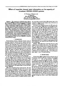
Fig. 2.
b) With index k ∈ j = 1, ..., lu , there is an associated index set c Dk such that c Dk ⊆ N k−1 , ´ ³ X x∗i = F k ∪ c Dk , k∪ c Dk
Partitioning of the index set.
Next we need to examine in more detail the structure of the optimal linear programming solution (11). According to (11), x∗k may take values less than or equal to αk . An index such that x∗k = αk is called “stable”, while an index such that x∗k < αk , “unstable”. We therefore have that for a stable index k, for any D ⊆ Nk−1 X αk ≤ F (k ∪ D) − x∗i . (35) D
Similarly, for an unstable index k, for any set Dk ⊆ Nk−1 such that X x∗i , x∗k = F (k ∪ Dk ) − Dk
it holds
F (k ∪ Dk ) −
X
x∗i < αk .
(36)
Dk
The general structure of the vector {x∗k }k∈N is as follows. The set of indices is partitioned into index sets Iis , i = 1, ..., ls , Iiu , i = 1, ..., lu such that ls • Indices in the set ∪i=1 I si are stable. Indices in the set lu u ∪i=1 I i are unstable. x • Index set Ii , x ∈ {s, u} consists of successive integers. x • If i > j then all indices in Ii , x ∈ {s, u} are larger x than the indices in Ij . Figure 2 shows an example of the partition of the index set for N = 10 channels. For convenience in the discussion we assume that for a given i, the indices in Iis are smaller than the indices in Iiu . Hence, for consistency, if index 1 is unstable, we define I1s = ∅. If k ∈ I uj then define bI k = ∪ji=1 I¯si . ¯ ¯ u u¯ Denote by u1 < u2 < ... < uL , L = ¯∪li=1 Ii ¯ the unstable indices. In the following, we assume that strict submodularity holds, i.e., whenever S − D 6= ∅ and D − S 6= ∅, it holds, F (S) + F (D) > F (S ∪ D) + F (S ∩ D),
(37)
therefore, whenever F (S) + F (D) = F (S ∪ D) + F (S ∩ D), then either S ⊆ D or D ⊆ S. This assumption is not essential but simplifies the proofs.
0-7803-7753-2/03/$17.00 (C) 2003 IEEE
for all D ⊆ Nk−1 ³ ´ X X bk − F k∪D x∗i ≤ F (k ∪ D) − x∗i , bk D
D
bk , and for all D ⊂ D ´ X ³ X bk − x∗k = F k ∪ D x∗i < F (k ∪ D) − x∗i . bk D
D
bui−1 ⊆ D bui , 2 ≤ i ≤ L. c) ui−1 ∪ D i−1 c d) Dui = ∪j=1 uj ∪ f Dui , where f Dui ⊆ bI ui , 1 ≤ i ≤ L. ek e) If k is an unstable index, then for any set S ⊆ Hk ≡ Ibk −D it holds ´ ´ ³ ³ X bk ∪ S − F k ∪ D bk . αi ≤ F k ∪ D S
f) If k is the´ largest index in I uj then for any set S ⊆ ³ bI k ∪ I sj+1 − f Dk it holds ´ ´ ³ ³ X αi ≤ F k ∪ c Dk ∪ S − F k ∪ c Dk . S
Proof: a)Let S ⊆ I1s and let k be the largest index in S. Then, since S − {k} ∈ Nk−1 , according to the definition of x∗k and I1s we have X αk ≤ F (k ∪ (S − k)) − αi S−k
or,
X S
(38)
αi ≤ F (S) .
b) According to the definition of x∗k , there is a set Dk ⊆ Nk−1 such that for all D ⊆ Nk−1 , X x∗k = F (k ∪ Dk ) − x∗i D
Xk x∗i . ≤ F (k ∪ D) −
(39)
D
Let Dk1 ⊆ Nk−1 be another set such that ¢ X ∗ ¡ x∗k = F k ∪ Dk1 − xi . 1 Dk
IEEE INFOCOM 2003
b um ⊆ D bui , which will prove part c), provided holds, um ∪ D that we also show that
Since by definition X ¢ X ∗ ¡ xi ≤ F (k ∪ Dk1 ∪ Dk ) − x∗i , F k ∪ Dk1 − D1
F (k ∪ Dk ) −
k X
Dk
D1 ∪Dk
k X ¡ ¢ x∗i ≤ F (k ∪ Dk1 ∩ Dk ) − x∗i , 1 ∩D Dk k
we have by adding and cancelling summation terms, F (k ∪ Dk ) + F (k ∪ Dk1 ) ≤ ¡ ¢ F (k ∪ Dk1 ∪ Dk ) + F (k ∪ Dk1 ∩ Dk ) =
bu D
By submodularity,
´ ³ bui ∪ um ∪ D bum − = F ui ∪ D
¡ ¢ F (k ∪ Dk ) + F k ∪ Dk1
= F (k ∪ Dk1 ∪ Dk ) + F ((k ∪ Dk1 ) ∩ (k ∪ Dk )).
This equality and the strict submodularity property imply that bk be the set either Dk ⊆ Dk1 or Dk1 ⊆ Dk . Let now D with smallest cardinality among those that satisfy (39). By definition, this set satisfies part b) of the lemma. Assume for the moment that part c) holds up to value i. Part d) for i = 1 follows from the definitions, and for i ≥ 2 it is immediate from c). We will also show that e) and f) hold. eui = Ibui − D bui ⊆ Nui −1 . To prove e), let S ⊆ Ibui − D Then, X X b ui ) − bui ∪ S) − F (ui ∪ D x∗j ≤ F (ui ∪ D x∗j , b u ∪S D i
bu = ∅, hence, taking into account that S ∩ D i X ∗ bu ∪ S) − F (ui ∪ D bu ). xj ≤ F (ui ∪ D i i
(40)
S
u To prove f) assume ³ that ui is ´the largest index in Ij and bu ) and let ik be − (ui ∪ D I s 6= ∅. Let S ⊆ Ibu ∪ I s j+1
i
j+1
i
bu and (40) the largest index in S. If ik ∈ Ijs then S ⊆ Ibui − D i s b , then since u ) ⊆ Nik −1 , holds. If i ∈ I ∪ D ∪ (S − i k i u k i j+1 ´ ³ bui ∩ (S − ik ) = ∅, we have from (35), and ui ∪ D bui ∪ (S − ik )) − αik ≤ F (ik ∪ ui ∪ D
X
bu ui ∪D i
bu ∪ S) − F (ui ∪ D bu ) − = F (ui ∪ D i i
x∗j −
X
X
αj
S−ik
αj ,
S−ik
where we used the fact that by part b) of the lemma, X bui ). x∗j = F (ui ∪ D bu ui ∪D i
That is,
X S
bui ∪ S) − F (ui ∪ D bui ). αj ≤ F (ui ∪ D
It remains to prove part c). Assume that part c) holds up to index i − 1. Assume also that for index um−1 , 1 < m < i it bu b holds um−1 ∪ D m−1 ⊆ Dui . We will show then that it also
0-7803-7753-2/03/$17.00 (C) 2003 IEEE
(41)
The proof of (41) will be outlined at the end, since it is basically a rewording of the argument for general m. bu ⊆ Nu −1 , bu ∪ um ∪ D Since D i m i ´ X ³ bui − F ui ∪ D x∗j i ´ ³ bui ∪ um ∪ D bum − ≤ F ui ∪ D
F (k ∪ Dk1 ∪ Dk ) + F ((k ∪ Dk1 ) ∩ (k ∪ Dk )).
bu D i
bu ⊆ D bu . u1 ∪ D 1 i
−
X
x∗j
X
x∗j
bu b u ∪um ∪D D m i
X
x∗j
bu um ∪D m
bu ) b u −(um ∪D D m i
´ ³ bui ∪ um ∪ D bum − F (um ∪ D b um ) = F ui ∪ D X x∗j . − That is
bu ) b u −(um ∪D D m i
X
x∗j
bu ) b u ∩(um ∪D D m i
bui ) + F (um ∪ D bum ) ≥ F (ui ∪ D bu ∪ um ∪ D bu ) − F (ui ∪ D i ´ ³ m ´´ ³³ b ui ∩ u m ∪ D b um (42) ≥ F ui ∪ D ³ ³ ´´ bu ∩ um ∪ D bu =F D , (43) i m ³ ´ bu − where in (42) the inequality is strict if ui ∪ D i ³ ´ ´ ³ ´ ³ bu bu bu 6= ∅. um ∪ D u ∪ D ∪ D = 6 ∅ and u − m i m m i Equality from the fact that since i > m, ³ (43) follows ´ bum = ∅. ui ∩ um ∪ D bum ⊆ Num −1 , bui ∩ D We also have since D ´ X ³ bu F um ∪ D x∗j − m bu D
m ³ ´´ ³ bu ∩ D bu ≤ F um ∪ D − i m
³ ´´ ³ bu ∩ D bu = F um ∪ D − i m
X
x∗j
bu b u ∩D D m i
X
x∗j + x∗um ,
bu ) b u ∩D um ∪(D m i
bui ∩ /D where in the last equality we used³ the fact that ´ umP∈ ∗ b b Dum . Since by part b), xum = F um ∪ Dum − Db u x∗j , m we conclude that ³ ´´ ³ X bui ∩ D bum , (44) x∗j ≤ F um ∪ D bu ) b u ∩D um ∪(D m i where in (44), by part b) of the lemma, the inequality is strict bu ∩ D bu ⊂ D bu . if D i m m
IEEE INFOCOM 2003
´ ³ bui . Then D b um = bui ∩ um ∪ D Assume now that um ∈ /D ´ ³ ´ ³ bum . Define Ebm = D bum − um−1 ∪ D bum−1 . b ui ∩ D b ui ∩ D D bum−1 ⊆ Since by the inductive assumption we have um−1 ∪ D b b Dui ∩ Dum , we can write X X x∗j = x∗j b u ∩(um ∪D bu ) D m i
= =
b u ∩D bu D m i
X Ebm
X Ebm
x∗j +
X
x∗j
bu um−1 ∪D m−1
³ ´ bum−1 . − F um−1 ∪ D
(45)
Observe that by the inductive hypothesis´ we have that Ebm ⊆ ³ s e b b eum−1 depending b Ium−1 −Dum−1 or Em ⊆ Ium−1 ∪ Ij+1 −D on whether um−1 is not, or is, the largest element in Iju . In either case have by e) and f) ´ ³ X X bu x∗j = αj ≤ F um−1 ∪ D ∪ Ebm m−1
Ebm
Ebm
´ ³ bum−1 −F um−1 ∪ D ´ ´ ³ ³ bu b bu ∩ D =F D ∪ D − F u m−1 um−1 . i m
(46)
Inequality (45) contradicts (46) and therefore we conclude bu . This implies that that um ∈ D i ³ ´ bui ∩ (um ∪ D bum ) = um ∪ D b ui ∩ D b um D From (43) and (44) it follows that ³ ´´ ³ X b ui ∩ D b um F um ∪ D x∗j ≥ b u ∩D bu ) um ∪(D m i ³ ´´ ³ b bu , ≥ F um ∪ Dui ∩ D m
b um ⊆ D bui . with equalities holding only if D To complete the proof we need to prove (41). For this we follow essentially the same arguments as above, by replacing Dum−1 with the empty set. m with 1 and um−1 ∪ c bui can be written According to parts b) and c) of Lemma 5, D i−1 eu , e b e b as Dui = ∪j=1 uj ∪ Dui , where Dui ∈ Iui . Let D ⊂ D i ¢ ¡ i−1 b hence ∪j=1 uj ∪ D ⊂ Dui . Applying part b) of Lemma 5 eui , we have and taking into account that x∗i = αi when i ∈ D ³ ´ X X eui − x∗j − αj F ∪ij=1 uj ∪ D ∪i−1 l=1 ul
eu D
i X X ¢ ¡ i ∗ < F ∪j=1 uj ∪ D − xj − αj ,
∪i−1 l=1 ul
0-7803-7753-2/03/$17.00 (C) 2003 IEEE
D
´ ³ X ¢ ¡ eui − F ∪ij=1 uj ∪ D < F ∪ij=1 uj ∪ D αi . e u −D D i
eu − D in the previous inequality we have the Setting S = D i following corollary. e ui , Corollary 6: If we set Ui = ∪ij=1 uj , then for any S ⊆ D S 6= ∅, it holds ³ ³ ´´ X ´ ³ eui − F Ui ∪ D eui − S αi . F Ui ∪ D < S
³ ´ bum−1 . x∗j + F um−1 ∪ D
bu and ui ∈ bu , from the strict submodularity /D /D Since um ∈ i m and (43) it follows that ´ ³ X bum bui ∩ D x∗j > F D Ebm
or
The next theorem provides the range within which each of the queues in N fluctuates. Theorem 7: Under policy π∗ , if qi (0) = 0, i ∈ N , then u for T large enough, the queues in ∪L i=1 Ii tend to infinity. eu0 = ∅, we have for a number M = O, Moreover, setting D max
{qi (t)} ≤ (N + 1 − uj )T + M for all t ≥ 0,
min
{qi (t)} ≥ (N + 1 − uj )T − M for all t ≥ τ 0 ,
eu e u −D D j j−1 e u −D eu D j j−1
eu , max ls s e qi (t) ≤ M for all t. It and if i ∈ / D L ∪j=1 Ij −DuL suffices to take T > 2M. In the course of the proof of Theorem 7 we also prove the main result of this paper, that is, Theorem 8: The throughputs achieved by policy π∗ for T large enough, satisfy the resurcive equations ( ( )) X x∗k = min αk , min x∗i F (k ∪ D) − , D⊆Nk−1
D
for k = 1, ..., N. Proof: In Lemma 2 set D = I1s , H = (N + 1 − u1 )T, Φ = T, and L = ∅. Conditions a), b) of the lemma hold because of the definition of policy π∗ . From Lemma 5 we have that condition c) holds as well. Since condition d) of the lemma also holds by the assumption that qi (0) = 0, i ∈ N , we conclude that for all t ≥ 0, maxs {qi (t)} ≤ (N + 1 − u1 )T + O i∈I1
(47)
provided that T ≥ O. Since Bi (0, t) = Ai (0, t) − qi (t), from (47) we conclude that for i ∈ I1s , Bi (0, t) Ai (0, t) ri = lim (48) = lim = αi = x∗i . t→∞ t→∞ t t eu1 ⊆ I1s we have from (36) and the b u1 = D Since D s definition of I1 that X e u1 ) − F (u1 ∪ D α i < α u1 . (49) eu D 1
Observe that X qj (t) = Au1 ∪De u (0, t) − Bu1 ∪De u (0, t) eu u1 ∪D 1
1
1
≥ Au1 ∪De u (0, t) − Cu1 ∪De u (0, t) 1 1 X eu ) t − O, αi − F (u1 ∪ D ≥ 1 eu u1 ∪D 1
IEEE INFOCOM 2003
that is, ru1 = x∗u1 . Using similar arguments we can show the claims for the rest of the queue indices.
and taking into account (49) we conclude that X qj (t) = ∞. lim t→∞
eu u1 ∪D 1
eu1 ⊆ I1s , we conclude Since by (47) qi (t) is finite for i ∈ D that limt→∞ qu1 (t) = ∞. eu1 it holds According to Corollary 6, for any subset S ⊆ D ³ ³ ´´ ´ ³ X e u − F u1 ∪ D eu − S . αi > F u1 ∪ D 1 1 S
eu ⊆ I1s , by the definition of the queue Notice that since D 1 eu1 are served according to the indices Ii (q) the queues in D LCQ policy when they are smaller than H = (N + 1 − u1 )T. Moreover, since limt→∞ qu1 (t) = ∞, it holds that Iu1 (qu1 (t)) = H, for t larger than or equal to some time t0 . Hence, for t ≥ t0 queue u1 has priority over the queues eu1 whenever maxi∈S {qi (t)} ≤ H. Therefore, in S ⊆ D eu and we can apply Lemma 4 with L = u1 , D = D 1 H = (N + 1 − u1 )T to conclude that there is some time eu1 , and for all t ≥ τ 10 , it holds τ 10 ≥ t0 such that for i ∈ D min {qi (t)} ≥ (N + 1 − u1 )T − O.
eu i∈D 1
(50)
From Lemma 5, e) it follows that for any subset S ⊆ E1 = eu (E1 = I s ∪ I s − D eu if u1 is the only element in I1s − D 1 2 1 1 I1u ) it holds ´ ´ ³ ³ X eu1 ∪ S − F u1 ∪ D e u1 . αi ≤ F u1 ∪ D S
Applying now Lemma 2 with D = E1 , H = (N + 1 − u2 )T , eu1 , we conclude that for all t ≥ 0, Φ = T and L = u1 ∪ D max {qi (t)} ≤ (N + 1 − u2 )T + O i∈E1
provided that T ≥ O. Pick now T large enough so that T − O > O.
(51)
(52)
Then since u2 > u1 , it holds
(N + 1 − u1 ) T − O > (N + 1 − u2 ) T + O.
(53)
Inequalities (50), (51) and (53) and the fact that qu1 (t) → ∞, ( i.e., Iu1 (qu1 (t)) = (N + 1 − u1 ) T, for t ≥ τ 10 ) imply that eu have higher priority over the rest of the the queues in u1 ∪ D 1 1 queues for t ≥ τ 0 and that they are nonempty. Therefore, the eu use all the available channel slots. Since queues in u1 ∪ D 1 Bu1 ∪De u (τ 10 , t) = Cu1 ∪De u (τ 10 , t), 1
1
we conclude that Bu1 ∪De u (0, t) Cu1 ∪De u (0, t) 1 1 = lim . lim t→∞ t→∞ t t Taking into account (48) and the fact that ´ ³ Cu1 ∪De u (0, t) 1 eu1 , lim = F u1 ∪ D t→∞ t we conclude that limt→∞ (Bu1 (0, t)/t) exists and ³ ´ X Bu1 (0, t) bu1 − αi , ru1 = lim = F u1 ∪ D t→∞ t
V. C ONCLUSIONS We presented a policy for scheduling packets for transmission over channels with time varying connectivity. We showed that the proposed policy maximizes the weighted sum of channel throughputs under any packet arrival rates. We adopted a burstiness-constrained channel model for the analysis. This model facilitates the analysis, while at the same time allows us to dispose of statistical assumptions. In this paper, we restricted ourselves to the case where the channels are in one of two states, “on” and “off”. A subject of further work is to generalize our approach to include the case of multi-rate channels. Another subject of ongoing work is to generalize our approach to include more general optimization functions. Furthermore, the consideration of packet delays, in addition to throughput, is a practical matter that needs to be addressed. R EFERENCES [1] C. S. Chang, Performance Guarantees in Communication Networks, Springer Verlag, 2000. [2] R. L. Cruz, “A calculus of delay Part I: Network element in isolation", IEEE Trans. Inform. Theory, vol 37, pp 141-131, Jan 1991. [3] R. L. Cruz, “A calculus of delay Part II: Network analysis”, IEEE Trans. Inform. Theory, vol 37, pp 132-141, Jan. 1991. [4] Bedekar, A., Borst, S.C., Ramanan, K., Whiting, P.A., Yeh, M., ”Downlink Scheduling in CDMA Data Networks”, Proc. IEEE Globecom 1999, pp. 2653-2657. [5] P. Bhagwat, P. Bhattacharya, A. Krishna, S. Tripathi, ”Enhancing Throughput over Wireless LANs using Channel State Dependent Packet Scheduling”, Proc. IEEE Infocom 97, April 1997. [6] Sem Borst, Phil Whiting, ”Dynamic Rate Control Algorithm for HDR Throughput Optimization”, IEEE Infocom 2001. [7] M. Grotschel and L. Lovasz, A. Schrijver, Geometric Algorithms and Combinatorial Optimization, Springer-Verlag, 1991. [8] Michael Neely, Eytan Modiano and Charles Rohrs, ”Power and Server Allocation in a Multi-Beam Satellite with Time Varying Channels,” IEEE Infocom 2002, New York, June, 2002. [9] Xin Liu, Edwin K. P. Chong, Ness B. Shroff, “Transmission Scheduling for Efficient Wireless Network Utilization”, Infocom 2001, Anchorage, Alaska, pp 776-785, 2001 [10] E. Seneta, Non-negative Matrices and Markov Chains, Springer-Verlag 1980. [11] Sanjay Shakkottai and Alexander Stolyar, “Scheduling for Multiple flows Sharing a Time-Varying Channel: The Exponential Rule”, To appear in Transactions of the AMS, A volume in memory of F. Karpelevich, Providence, R.I.: American Mathematical Society, 2001. [12] L. Tassiulas and A. Ephremides, “Dynamic Server Allocation to Paraller Queues with Randomly Varying Connectivity”, IEEE Trans. on Information Theory, vol 39, no 2, March 1993. [13] L. Tassiulas. “Scheduling and performance limits of networks with constantly changing topology,” IEEE Transactions on Information Theory, Vol. 43, No. 3, pp. 1067-1073, May 1997.
bu D 1
0-7803-7753-2/03/$17.00 (C) 2003 IEEE
IEEE INFOCOM 2003