Exploration and Map-Building under Uncertainty with ... - cse.sc.edu

2011 IEEE International Conference on Robotics and Automation Shanghai International Conference Center May 9-13, 2011, Shanghai, China

Exploration and Map-Building under Uncertainty with Multiple Heterogeneous Robots Lourdes Mu˜noz-G´omez†, Moises Alencastre-Miranda†, Rigoberto Lopez-Padilla‡ and Rafael Murrieta-Cid‡ †Tecnol´ogico de Monterrey Campus Santa F´e, M´exico {lmunoz,malencastre}itesm.mx

‡Centro de Investigaci´on en Matem´aticas, CIMAT Guanajuato, M´exico {rigolpz,murrieta}@cimat.mx

Abstract— In this paper, we present a multi-robot exploration strategy for map-building. We consider a team of robots with different sensing and motion capabilities. We combine geometric and probabilistic reasoning to propose a solution to our problem. We formalize the proposed solution using dynamic programming in states with imperfect information. We apply the dynamic programming technique in a reduced search space that allows us to incrementally explore the environment. We propose realistic sensor models and provide a method to compute the probability of the next sensor reading given the current state of the team of robots based on a Bayesian approach.

I. I NTRODUCTION Automatic environment exploration and map building is an important problem in mobile robotics. Autonomous robots must posses the ability to explore their environments, build representations of those environments (maps), and then use those representations to navigate effectively. Maps built upon exploration can be used later by the robot to perform other tasks such as object finding. A strategy for exploring an unknown environment and building an environment representation with a mobile robot can be performed as follows: (i) the robot builds a local map with the sensor readings (ii) the robot moves to an intermediary goal, which is defined based on suitable properties (iii) a global map is updated merging the information between the current global map and the new local map. In the last two decades several approaches have been proposed for map-building, for instance [5], [8], [10], [19] just to name a few. Most previous research has focused on developing techniques to extract relevant information from raw data and to integrate the collected data into a single model. However, a robot motion strategy to explore the environment has been less studied. In this work, we deal mainly with this latter problem. In this paper an exploration strategy is proposed. Our exploration strategy considers sensing and motions capabilities of each robot. Our algorithm outputs the sensing configurations to be visited. The sensing configurations are associated to the borders between the known and unknown space. Our method assigns a robot of the team for visiting a selected sensing configuration, according to its capabilities and without considering predefined roles. Our main contributions are: (1) We consider a team of robots with different sensing and motion capabilities. (2) We formalize the proposed solution using dynamic programming 978-1-61284-380-3/11/$26.00 ©2011 IEEE

in states with imperfect information. (3) We propose realistic sensing models. (4) We propose a method to compute the probability of the next sensor reading given the current state based on the Bayes rule. II. R ELATED W ORK Several robot exploration strategies for map building have been proposed. It is possible to classify those exploration strategies into two main types: (i) systematic exploration and (ii) strategies in which sensed information is taken into account to define the next sensing location. In systematic explorations, the robots follow a predefined motion pattern, for instance following walls [3], moving in concentric circles [15], and so forth. In non-systematic exploration, information taken by the sensor is frequently used to select an appropriated sensing location. A common strategy is the frontier-based exploration, originally proposed by Yamauchi in [23]. In this strategy to explore the environment, the robot goes to the imaginary line that divides the known and unknown parts of the environment. In [16], [11], [13], the proposed exploration strategies lead the robot to locations in which maximal information gain is expected, a cost function is defined to maximize the new information that will be obtained in the next sensing location. Several works have proposed to generate random sensing locations and then evaluate them to select one that maximizes a cost function. The exploration strategy presented in [12] is based on the computation of the next best view and the use of randomized motion planning. In [12] the proposed motion strategy only considered the case of a single robot. In [1] an interesting experimental evaluation of several exploration strategies is presented. However, in that work the case of multi-robot exploration is not studied. Some works have proposed multi-robot exploration and mapping [17], [7]. In both of these works, the information gain and the exploration cost are considered simultaneously to define the next locations for each robot of the team. In [7] the map is represented using an occupancy grid and the possible locations for the next exploration step are defined over cells lying on the border between the known and unknown space. In [22] the authors propose a multi-robot exploration strategy in which instead of frontiers, the authors use a segmentation of the environment to determine exploration

2295

targets for the individual robots. This segmentation improves the distribution of the robots over the environment. We have already proposed motion strategies for exploration and mapping. In [21] we have presented techniques that allow one or multiple mobile robots to efficiently explore and model their environment. We developed a utility function that measures the quality of proposed sensing configurations, and a randomized algorithm for selecting the next sensing configuration. In that work we have considered a team of homogeneous robots (same sensing and motion capabilities). Some previous works have already proposed exploration with multiple robots having different capabilities. The work presented in [18] considers a team composed by robots of different sizes. During the exploration, if a robot is too big to navigate among obstacles and reach a sensing location, then it asks to a smaller robot to perform the task. In [9] robots have one of two roles: Navigator or cartographer, navigators randomly move in the environment until they find a target location for a cartographer, after that the cartographer moves to the target location. In the works mentioned above each robot follows a specific and predefined role according to its type. In this work, we propose motion strategies for exploration and map building considering the robots capabilities, but we do not assign pre-defined roles to the robots of the team, instead, we model the robots capabilities probabilistically. III. P ROBLEM D EFINITION , N OTATION AND A PPROACH OVERVIEW The problem addressed in this paper consists in exploring an unknown environment and incrementally building a model of that environment with a team of mobile robots having different sensing and motion capabilities. We assume that the sensors and motors of each robot are imprecise. Our goal is to propose a robot motion strategy, which generates a fast and reliable map building. We also want to profit the most of the different capabilities of each robots according to the exploration and map building tasks. We propose a discrete time approach and consider a team with n robots. To explore the environment as quickly as possible, sensing configurations that provide maximal view of unexplored areas should be preferred. Hence, we use a frontier-based exploration. Points belonging to the obstacles (discrete sensor reading) are obtained by a sensor (e.g. a laser range finder). Every point is denoted sj ∈ R2 . The ensemble of points is denoted [ sj S= j

This ensemble is a set. Based on this set, obstacles can be model with poly-lines applying a line fitting technique [21] over the sensed points. This step is needed to facilitate visibility computations. Visibility computation (which yield visibility polygons) over the sensed environment is used to define the borders between the known and unknown environment. We denote by V (qi ) a visibility polygon of robot i at configuration

qi ∈ R2 × SO(2). We consider disk robots, a robot is free to move in the interior of its visibility polygon, so long as it does not collide with an obstacle. We denote by F (qi ) the visibility polygon reduced by the robot radius, i.e., F (qi ) is a safe region for navigation that is visible from configuration qi . We define Vtot as the total visibility region for the team of robots, and Ftot as the total visible region in which any robot can move, i.e., [ [ F (qi ). V (qi ) and Ftot = Vtot = i

i

A frontier (free edge) is defined as the border between the visibility region V (qi ) and the unseen environment. Local maps are composed by points (the original sensor readings signaling the obstacles) and by frontiers. Thus, while the local maps contain free edges, the robots have not finished the exploration. Indeed, our local maps are located at the border between the known and unknown environment. The local maps are denoted S tp (q(i,k) ). They are related to the robots configurations q(i,k) , k indexes the time step in which the local map is sensed, i the robot, and tp ∈ N denotes a type of local map (we consider that there are different types of local maps, more details are given below). Let C, U and Z respectively denote the configuration, control and observation spaces, which respectively correspond to all possible robots configurations, controls and sensor readings. The state space is X ⊂ C × E, E is the set of all possible environments in which the robots might be. Evidently, there is a relation between the state xk and the robots observation state zk . Thus, zk = h(xk ), zk ∈ Z, xk ∈ X and q(i,k) ∈ C. Based on sampling, we generate candidate sensing configurations over the configuration space C. The samples are only generated close to the free edges. Besides, only the samples inside Ftot are considered. Thus, visibility computations are used to bias the sampling. Since selected samples are close to the border between the explored and unexplored environment, they have a good chance of seeing unknown environment. The robots move following only two motion primitives: Rotation in site without translation and straight line motions. Between two configurations q(i,k) , q(i,k+1) , the robot path is composed by 3 motion primitives. First, the robot rotates aiming to the goal. Second, it translate to this goal. Finally, the robot rotates again to reach its final orientation. The resulting robot path lies totally inside F (qi ), and hence, it is not needed to be tested for collision. For multiple robots, the motion primitives are the same for each robot. Furthermore, the exploration starts assuming that Ftot has a single connected component. In general, if a robot i of the team has to visit a candidate sensing configuration of another robot j then it might not be possible for the robot i to travel between the two configurations by following a straight line. In those cases, we use a reduced visibility graph (computed over C) to follow the shortest path between the sensing configuration. The resulting path is totally inside Ftot .

2296

We deal with uncertainty in both sensing and control. We model this uncertainty using probabilistic methods. We assume that each robot has its own control model that indicates the probability of reaching a next state xk+1 from a current state xk applying some controls uk ∈ U. We denote this probability p(xk+1 |xk , uk ), which probabilistically take the robots to the next state xk+1 . The relation between p(xk+1 |xk , uk ) and the inaccuracy of the control uk can be found in [20]. We assume that our robots are equipped with sensors having different range, resolution, and different precision to determine the distance from the robot to the obstacles. Since, we want to incrementally build a map of the environment, we need to find the best alignment between the current sensor reading and the new one. We used original data to align local maps with the global one. The best transformation according to the Hausdorff distance is used to correct the robot position and merge the maps. But, at the end the stored map is composed of polylines obtained through line fitting of the sensor reading [21]. Inspired by Bayesian approaches, we propose to use a priori information of the environment, which can be incorporated to our models to make better decisions. We define the mapping zk+1 = h(xk+1 ) between the observation state zk+1 and the system state xk+1 . This mapping h(xk+1 ) is simply defined as an equivalent relation zk+1 ∼ tp. This is useful, because it provides a manner to estimate the sensor reading zk+1 given the state xk+1 . p(zk+1 |xk+1 ) denotes the probability of the observation state zk+1 given the system state xk+1 . The Bayes rule is used to calculate it. In this setting, p(xk+1 |zk+1 ) can be estimated using a nearest neighbor method. Since a local map is a set of points, we use the Hausdorff distance as metric in the nearest neighbor method to measure the resemblance between the sets S tp (related to the observation state zk+1 ) and a hypothesized set S(k+1) (related to the system state xk+1 ). We estimate the type of local map tp that we would obtain as sensor reading zk+1 . For a set of explorer robots, the system can be modeled as a dynamic system. The system evolves from an state to another while robots of the team move to frontiers. The system information state is defined as Ik = (u1 , . . . , uk−1 , z1 , . . . , zk ). Ik is the history of all sensor readings until time k and all controls that have been applied to the system until time k − 1. Dynamic programming is used to select the next sensing configuration considering the information state Ik [4]. IV. M ODELING A S OLUTION W ITH DYNAMIC P ROGRAMMING Since, we assume uncertainty in both sensing and control, we model our problem as a dynamic system with imperfect information state. Our dynamic system is defined as follows: • The set of possible states is denoted as X , for n robots a state is x = (x1 , . . . , xi , . . . , xn )T , x1 , xi and xn respectively denote the state of robot 1, robot i and

robot n. We assume mobile robots with 3 degrees of freedom, so the configuration of each robot i is a vector qi = (px , py , θ)T , px and py denote the robot position in a two dimensions global reference frame, θ denotes the robot orientation with respect to the abscissa axis in the global reference frame. We consider that a robot state xi is equivalent to a robot configuration qi × e, e ∈ E denotes the environment in which the robot is. The environment e is represented as a set of local maps [ S(q(i,k) ) e= (i,k)

•

•

•

The set of possible controls is denoted U, each element of the set ui ∈ U is a vector having the controls for each robot. We consider differential drive robots. The set of possible readings taken by the robots sensors is Z, zi ∈ Z is a vector, which includes the sensor reading of each robot. We use probabilistic modeling. The system changes from a state xk in time k to another state xk+1 after having applied control uk with probability p(xk+1 |xk , uk ). Since there are n robots, we have a probability p(x(i,k+1) |x(i,k) , u(i,k) ), in which i denotes the i − th robot. We assume this probability independent for each robot. Therefore, we have: p(xk+1 |xk , uk ) = p(x(1,k+1) |x(1,k) , u(1,k) ) . . . p(x(n−1,k+1) |x(n−1,k) , u(n−1,k) )p(x(n,k+1) |x(n,k) , u(n,k) )

•

In this paper we consider those probabilities given. p(zk+1 |uk , xk+1 ) is the probability of obtaining a sensor reading zk+1 given that the system is at state xk+1 , having applied control uk . We assume that the sensor reading zk+1 is independent of the control uk . It means that robots sense the environment, when they are motionless, after reaching a given sensing configuration. Hence, p(zk+1 |xk+1 , uk ) = p(zk+1 |xk+1 ). Furthermore, we also assume these probabilities independent for each robot, thus: p(zk+1 |xk+1 ) = p(z(1,k+1) |x(1,k+1) )p(z(2,k+1) |x(2,k+1) ) . . . p(z(n,k+1) |x(n,k+1 ))

In Section IV-C we propose a Bayesian approach to estimate p(zk+1 |xk+1 ). We apply dynamic programming in the system defined above to obtain the optimal action to be executed. We consider all the information available: History of both controls and sensor reading. Thus, we select the action to be executed at time k based on Ik . The dynamic programming equation considering Ik is given by equation 2 [4]. Jk (Ik ) = max[g(Ik , uk ) + E{Jk+1 (Ik , zk+1 , uk )|Ik }] (2) uk

In equation 2, g(Ik , uk ) represents the utility (gain over cost) of applying a given action. It indicates how useful it

2297

p(xk+1 |Ik+1 ) = P

P

p(xk |Ik )p(xk+1 |xk , uk )p(zk+1 |uk , xk+1 ) P xk p(xk |Ik )p(xk+1 |xk , uk )p(zk+1 |uk , xk+1 ) xk+1 xk

is to apply a control uk in which the information vector is Ik (history of both controls and sensor reading). g(Ik , uk ) can be calculated in terms of g(xk , uk ) with the following equation [4]. g(Ik , uk ) =

X

p(xk |Ik )g(xk , uk )

(3)

(1)

do consider as an option to send a robot to a frontier that is sensed by another robot. A. Objective function g(xk , uk ) g(xk , uk ) indicates how useful it is to apply a control uk given that the the system is at state xk .

xk

Area

Since we consider uncertainty, g(Ik , uk ) depends on both p(xk+1 |Ik+1 ) and g(xk , uk ). While the dynamic programming equation 2 is evaluated backwards, starting with the last step, the equation 1 is evaluated forwards beginning with k = 0. Notice that the dynamic programming technique considers all possible states (assuming that all the information is available from the beginning). However, in our setting, we do not have all the information at time k = 0. Besides, we want to incrementally explore the environment and build a global map. Consequently, when we make the decision of applying control uk and thus changing the system from state xk to xk+1 , we commit with that decision and we move the robots to obtain new information. In some future state, the possibles actions which consider robot motions different to the ones already executed are not considered. In our motion strategy, we do the following: (1) we consider p(xk+1 |Ik+1 ) to generate the action uk , and (2) we make short term plans. The first point means that, we do consider statistic of the history of past actions and sensors readings. Indeed, in [2], it has been shown that this is sufficient statistic of the information state. The second point means that, we only plan the action to change a state from k to k + 1, we do not plan a long order for visiting free edges. For instance, for a team composed by two robots (robot A and robot B), a state k transits to the next state k + 1, whenever one of the three following options happens: 1) robot A moves twice and robot B does not move, 2) robot B moves twice and robot A does not move, or 3) robot A moves once and robot B also moves once. The reason for generating short term plans is that we have previously shown [21] that making long term plans with partial and dynamic information will often result in a waste of resources. Notice that as soon as new frontiers (free edges) appear (which have not been considered in the original plan), the robot might need to come back to some configurations near to other configurations already visited, thus traveling longer than required. Changing a state from k to k + 1 might imply that all the robots of the team move. In order to facilitate the motion coordination of the robot’ team and avoid collision among them, we impose that a motion for a given robot j starts until the motion of other robot i is finished. However, we

Distance

Fig. 1.

Expected discovered area and traveled distance.

For each robot we define g(xi,k , ui,k ) as a function depending only on two factors (other functions depending on more factors, which might yield more realistic setting, can also be used in our formulation). These two factors are: (1) The new area A(q(i,k+1) ) that the robot can perceive at a next configuration. (2) The distance the robot would travel to reach that configuration d(q(i,k) , q(i,k+1) ). Figure 1 shows a robot at a configuration near to the border between the known and unknown environment. The circle around the robot depicts the area within the sensor range (the radius of the circle represents the sensor range). The shaded area is the maximum new area that the robot can discover at that configuration. We use the global map at time k to eliminate portions of this area that we know are obstacles already sensed [12]. We define g(xk , uk ) as an objective function that relates the utility (ratio of gain over cost) of the action with the control uk given the current state xk . g(xk , uk ) = g(x(i,k) , u(i,k) ) =

A(q(i,k+1) ) d(q(i,k) , q(i,k+1) )

(5)

Equation 4 defines the distance between configuration q(i,k) and configuration q(i,k+1) , in which α = min{|θ(i,k) − θ(i,k+1) |, 2π − |θ(i,k) − θ(i,k+1) |} B. Computing p(xk+1 |Ik+1 ) First, equation 1 is calculated to apply the dynamic programming equation. p(xk+1 |Ik+1 ) represents the probability of being in a state xk+1 considering the applied controls and sensed data. This equation is used in [20] to calculate the bel

2298

d(q(i,k) , q(i,k+1) ) =

q (px (i,k) − px (i,k+1) )2 + (py (i,k) − py (i,k+1) )2 + α2

in Bayes Filter and in [14] for representing a mapping on probabilistic information spaces. The equation 1, can be obtained from the Bayes’ rule, applying joint probability methods and marginalization. p(xk+1 |Ik+1 ) is expressed in terms of p(zk+1 |xk+1 , uk ), p(xk+1 |xk , uk ) and p(xk |Ik ). As it was mentioned above, we assume p(zk+1 |xk+1 , uk ) = p(zk+1 |xk+1 ). Indeed, we estimate p(zk+1 |xk+1 ) without actually taking the robot to state xk+1 , but computing its hypothesized visibility region (see figure 1). In fact, we make a prediction from state xk . To compute p(xk+1 |Ik+1 ), p(x0 |I0 ) is needed at the first step. At the beginning, no control has been applied and the only sensor reading is z0 , therefore I0 = z0 and p(x0 |I0 ) = p(x0 |z0 ). This probability is directly estimated using the nearest neighbor method described in the next Section.

(4)

the partial Hausdorff distance considering a transformation including both translation and rotation. Given two sets of points S tp = P and S(k+1) = Q, the partial Hausdorff distance is defined as (see [21]): H(P, Q) = max(h(P, Q), h(Q, P ))

(9)

h = Mp∈P min kp − qk

(10)

where q∈Q

where Mp∈P f (p) denotes the statistical mean value of f (p) over the set P and k.k is the Euclidean metric for measuring the distance between two points p and q. Thus, the Hausdorff distance is computed between the set S(k+1) and the five types of local maps S tp .

C. Estimating the probability p(zk+1 |xk+1 ) of the next sensor reading given the state We want to estimate the probability of the next sensor reading zk+1 , given that the robots are in the state xk+1 . We assume this probability independent of the controls uk . The Bayes rule is used to estimate p(zk+1 |xk+1 ). p(zk+1 |xk+1 ) = P

p(xk+1 |zk+1 )p(zk+1 ) xk+1 p(xk+1 |zk+1 )p(zk+1 )

ζ ntp φtp

(7)

ζ is the ζ − th nearest neighbor, ntp is the number of elements used in a training set belonging to the local map of type tp, and φtp is the surface that assigns a class (type of local map). For a training set in a feature space with a single characteristic, φtp is defined by: φtp = 2rtp

a)

b)

c)

(6)

We assume that the environment contains a bounded number of local map’ types. tp denotes a type, the local maps are sets of points obtained with a sensor (e.g. a laser range finder). The robots are provided with a training set of local map’ types. Each type itself has associated a probability of being sensed p(zk+1 ). In the absence of information this probability can be set equal for all types, or it can be obtained from supervised learning process. p(xk+1 |zk+1 ) is estimated using the nearest neighbor method [6]. p(xk+1 |zk+1 ) =

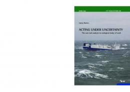
Local map of type single wall Local map of type corridor Local map of type corner

Local map of type T

d)

e)

Fig. 2.

Types of local maps S tp .

Figure 2 shows the five types of models that we use. We consider this five models as typical for an indoor structured environment. The dots represent the sensor reading. We use models with different number of points to simulate robots equipped with sensors having different resolutions, and the training data consider some variants of each one of the five main patterns (types of local maps) shown in figure 2. Obviously, our approach has the disadvantage that other types of local maps can appear. However, the type of map is only used for selecting the most appropriated robot according to its sensing and motion capabilities. At the end, the local map integrated to the global map corresponds to the actual sensor readings.

(8)

In this last equation rtp is the distance to the ζ −th nearest neighbor. Since a local map is a set of points, we use the partial Hausdorff distance as metric rtp , in the nearest neighbor method to estimate the resemblance between the sets S tp (related to the observation state zk+1 ) and the hypothesized set Sk+1 (related to the system state xk+1 ). We evaluate

Local map of type intersection

V. S IMULATIONS RESULTS In this section, we present simulation results. All our simulation experiments were run on a quad-core processor PC, equipped with 3 GB of RAM, running Linux. Our software is written in C++. For distinguishing the robots, in all the figures robot R1 is shown with a square and robot R2 with a circle, however for finding collision free paths both robots are modeled as disks

2299

a)

a)

b)

b) c)

d)

e)

f)

c) Fig. 4.

d)

e) Fig. 3.

Exploration 1

Exploration 2

with the same radius. In all simulation the visibility region of both robots is computed used a polygonal approximation of the data points obtained with the sensor. The visibility region of robot R1 is shown in dark gray (green) and the visibility region of robot R2 is shown in light gray (yellow). In the first experiment (figure 3), robot R1 has better sensing capabilities, but worse control capabilities compared with robot R2. That is, the robot R1 is equipped with a sensor having bigger range and better resolution than robot R2, However R1 has a associated probability of reaching the next state to which the robot is sent smaller than robot R2. In figure 3 an indoor environment (office type) is shown. The environment is 3000 units long and 2300 wide. The probability for reaching the next state p(xk+1 |xk , uk ) is set 0.2 for robot R1, and 0.9 for robot R2. Robot R1 has a sensing range of 1200 units and R2 has a range of 800 units. The sensor’s resolution of robot R1 is set to 2 degrees, and the sensor of robot R2 has a resolution of 4 degrees. Furthermore, the sensor of robot R1 may produce 2300

an error over the sensed distance to the obstacles bounded by 2 units, and the sensor of of robot R2 may produce an error bounded by 4 units. In this environment, we have run 20 simulations with the same initial robots configurations. Figure 3 a) shows the initial robots’ configurations, figures 3 b), 3 c) and 3 d) show snapshots of one of these experiments. In average, R1 has moved 4 times and robot R2 3 times to explore the environment. 15 over 20 times the following happened: robot R1, the one with better sensing capabilities, was selected to explore the richer visual local maps (left part of the environment) and robot R2 (having better control capabilities) was selected to explore local maps composed only by two parallel lines, the corridor in the right part of the environment (See figures 3 c) and 3 d)), which are hard to be matched with the global map. Notice that in corridors bounded with parallel featureless walls, a matching procedure only finds an alignment between the local and global maps, in the direction perpendicular to the walls. Figure 3 e) shows the sensed points collectively obtained by both robots. Based on these first results, we conclude that our approach generates robot behaviors, that is, robots with good sensing capabilities are selected to explore visually rich local maps, and robots with good control capabilities are used to explore local maps, which are hard to be matched with the global map. However, we plan to test our algorithms in real robots to verify this result. Figure 4 shows an environment with holes. In this environment, we have run a simulation in which both robot R1 and robot R2 have exactly the same sensing capabilities, but robot R2 has better control than robot R1. p(xk+1 |xk , uk ) is 0.5 for robot R1, and 0.7 for robot R2. In this simulation, robot R2 has moved 5 times and robot R1 has only moved twice. Furthermore, the total length of the path traveled by robot R1 is significantly smaller than the one traveled by robot R2. Finally, we stress that in all our simulations ran over the environments shown in figures 3 and 4, our software has found a plan to explore the whole environment in less than a minute. VI. C ONCLUSION AND F UTURE W ORK In this paper we have proposed a multi-robot exploration strategy for map-building. We have considered a team of non-identical robots; in particular, robots have different capabilities in both sensing and control. We have formalized our solution using dynamic programming in states with imperfect information. We have applied the dynamic programming technique considering a reduced search space, in which we avoid to consider unnecessary robot’ motions that could arise from a lack of knowledge about the unexplored part of the environment. This strategy greatly reduces the number of operations needed to evaluate the dynamic programming equation and allows us to incrementally explore the environment. We have also proposed a Bayesian method to estimate the probability of the next sensor reading given the state of the team of robots. As future work, we plan to obtain simulation results with a bigger number of robots, we would

like to analyze unsupervised learning algorithms to adapt the types of local maps during the exploration. Finally, we also want to test our approach in real robots. R EFERENCES [1] F. Amigoni, Experimental Evaluation of Some Exploration Strategies for Mobile Robots. In Proc. of IEEE International Conference on Robotics and Automation, 2008, pp 2818-2823. [2] K.J. Astrom, Optimal Control of Markov Processes with Incomplete State Information. In Journal of Math. Anal. Appl, 10, pp. 174-205, 1965. [3] A. Bemporad, M. DiMarco and A. Tesi, Wall Following Controllers for Sonar-Based Mobile Robots. In Proc. of Conference on Decision and Control, San Diego, CA, USA, 1997, pp. 3063-3068. [4] D. Bertsekas. Dynamic Programming and Optimal Control, Athena Scientific, 2000. [5] H. Bulata and M. Devy, Incremental construction of landmark-based and topological model of indoor environments by a mobile robot. In Proc. of IEEE International Conference on Robotics and Automation, 1996. [6] R. Duda and P. Hart, Pattern Classification and Scene Analysis John Wiley And Sons Inc, 1973. [7] W. Burgard, M. Moors, C. Stachniss and F.E. Schneider, Coordinated Multi-robot Exploration. In IEEE Transactions on Robotics, 21(3), 2005, pp. 376-386. [8] R. Chatila and J.-P. Laumond, Position referencing and consistent world modeling for mobile robots. In Proc. of IEEE International Conference on Robotics and Automation, St. Louis, USA, 1985, pp. 138-145. [9] W. Cohen, Adaptive mapping and navigation by teams of simple robots. In Journal of Robotics and Autonomous Systems, 18(4), 1996, pp. 411-434. [10] A. Elfes, Sonar-based real world mapping and navigation, In IEEE Transactions on Robotics and Automation, 3(3), 1987, pp. 249-264. [11] H. Feder, J. Leonard and C. Smith, Adaptive mobile robot navigation and mapping. In International Journal of Robotics Research, 18(1999) pp. 650-668. [12] H.H. Gonzalez-Banos and J.-C. Latombe, Navigation strategies for exploring indoor environments. In International Journal of Robotics Research, 21(10/11), 2002, pp. 829.848. [13] A. Makarenko, B. Williams, et. al. An experiment in integrated exploration. In Proc. of Int.IEEE/RSJ Conference on Intelligent Robots and Systems, 2002. [14] S. M. LaValle. Planning Algorithms. Cambridge University Press, 2006. [15] R. Sim and G.Dudek, Effective Exploration Strategies for the Construction of Visual Maps, In Proc. of Inter. Symposium on Intelligent Robots and Systems, Las Vegas, USA, 2003, pp. 3224-3231. [16] R. Sim and N. Roy, Global A-optimal Robot Exploration in SLAM. In Proc. of IEEE International Conference on Robotics and Automation, Barcelona, Spain, 2005, pp. 661-666. [17] R. Simmons, D. Apfelbaum, et. al. Coordination for multi-robot exploration and mapping. In Proc. of AAAI National Conference on Artificial Intelligence, 2000, pp. 852-858. [18] K. Singh and K. Fujimura, Map making by cooperating mobile robots. In Proc of International Conference on Robotics and Automation, 1993, pp. 254-259. [19] S. Thrun, W. Burgard and D. Fox, Probabilistic mapping of an environment by a mobile robot, In Proc. of International Conference on Robotics and Automation, 1998. [20] S. Thrun, W. Burgard and D. Fox, Probabilistic Robotics. MIT Press, 2005. [21] B. Tovar, L. Mu˜noz, R. Murrieta-Cid, M. Alencastre, R. Monroy and S. Hutchinson, Planning Exploration Strategies for Simultaneous Localization and Mapping, Journal Robotics and Autonomous Systems, Vol 54(4), April 2006, pp. 314-331. [22] K.M. Wurm, C. Stachniss, W. Burgard, Coordinated multi-robot exploration using a segmentation of the environment. In Proc. of IEEE/RSJ International Conference on Intelligent Robots and Systems (IROS 2008), Nice, France, 22-26 Sep, 2008, pp. 1160-1165. [23] B. Yamauchi, Frontier-Based Exploration using Multiple Robots, In Proc. of Inter. Conference on Autonomous Agents, Minneapolis, USA, 1998, pp. 47-53.

2301