Hybrid Lattice Particle Modeling of Dynamic Fracture Simulations of 2D Elastic Spring networks: Theoretical Considerations G. Wang 1 , A. Al-Ostaz 1 , A.H.-D. Cheng 1 and P. Raju Mantena 2 1
Department of Civil Engineering Department of Mechanical Engineering University of Mississippi University, Mississippi, 38677-1848, USA 2
Abstract This paper is concerned with the mathematical derivations of employing elastic interaction formula between contiguous particles in 2D lattice networks accounting for different types of linkage mechanism and different shapes of lattice. Axial ( α ) and combined axial-angular ( α - β ) models are considered together with triangular or rectangular lattice. Derivations are based on the equivalence of strain energy stored in a unit cell with its associated continuum structure in the case of in-plane elasticity. In this paper, a new hybrid lattice particle modeling (HLPM) scheme is proposed that considers different particle interaction schemes not only limited to the nearest particles but also extended to the particles in the second nearest neighborhood, and different mesh structures with triangular or rectangular unit cell. Conventional PM technique was restricted to a fixed Poisson ratio and had a strong bias in crack propagation direction, as dictated by the regular lattice structure employed. This HLPM is free from the abovementioned deficiencies and can be applied to a wide range of impact and dynamic fracture failure problems. Keywords: particle modeling, lattice model, dynamic fracture, impact, constitutive relations _____________________ * Corresponding author:
[email protected] (Ge Wang)
Tel: + 662 915 5369, fax: + 662 915 5523
1
1. Introduction Since its first presence in 1980’s [1], particle modeling (PM) technique has been constantly improved and has found good success in a number of applications including impact induced dynamic crack propagation and fragmentation [2-7]. In brief, the PM is a hybrid of Molecular Dynamic (MD) and the lattice modeling technique. It is based on lumped mass particles distributed on a lattice network, which have mass inertia and obey Newton’s second law of motion. It is a Lagrangian model that keeps track of particle location and velocity. The current PM technique [1-10] utilizes a popular lattice model by means of axial linkage in a 2D equilateral triangular lattice system. Only a nearest neighborhood of particles is defined for dynamic interaction. This treatment in both mesh and dynamic interaction is robust in solving solid problems. However, two main deficiencies are inherently derived, a fixed Poisson ratio equal to 1/3, and a bias related to the lattice geometry which results in preferential fracture propagation directions. To extend the PM to a wider extent of Poisson ratio as well as to eliminate the mesh bias problem, an attempt of employment of different mesh structures and/or particle interaction schemes is necessary. Since PM is run in lattice network, therefore, lattice model theory should be a help to this implementation. Research on spring network models (lattice models) started from more than 60 years ago [11]. Literature review on the successive development of these models can be found in [12–14]. Lattice modeling technique has been widely applied in the computation of effective elastic moduli and simulation of brittle intergranular fracture (BIF) in ceramics, intermetallics, and refractory metals [15-20]. However, since the conventional lattice technique is of an Eulerian model, it has been limited to static fractures and mostly applied in a microstructure system. To extend the success of lattice modeling to macroscopic and dynamic problems, it is ideal to develop a new dynamic model which is analogous to PM technique but can inherit the already-existing advantages of lattice model. To implement such a task, we first need to clarify the differences and correlations between lattice model and PM. Table 1 displays a comparison of these two models from some main aspects. In Table 1, we see that although these two models are quite different
2
from each other, both PM and lattice model may run with the identical mesh structure and have another overlap with interaction manner- spring connection, therefore our following modeling development work based on PM can benefit from the lattice modeling techniques associated with spring connections.
Table 1 Comparison of lattice model and PM Interaction Manner Interaction region Mesh Validation Poisson ratio extent Solution scheme
Lattice Model spring (axial/angular), beam, etc. not limited to nearest neighbor Eulerian (triangular, rectangular, etc) static in microstructure system various implicit (from force to displacement)
PM spring (axial only) nearest neighbor only Lagrangian (triangular, rectangular, etc) dynamic with multiscales fixed explicit (from displacement to force)
In the domain of lattice technique, fundamental research work has been completed in exploring the resultant effective elastic moduli and Poison ratio associated with some specific mesh structure and interaction scheme. For example, to eliminate the restriction of fixed Poisson ratio, Ostoja-Starzewski [14] has addressed the fundamental concepts of manipulating several types of lattice models, including central ( α ), angular ( β ) and the mixed ( α - β ) interactions, coupled with different lattice networks, triangular, rectangular, etc. If we transfer these lattice techniques into PM interaction, a more robust particle dynamics model will be born. However, the derivation that establishes the relation between the Poisson ratio and the spring coefficient under different lattice network and different coupling scheme was brief, and many practical issues relating to specific applications were not addressed. Thus, there is still much elaborately fundamental work to do. In this paper, we provide a detailed derivation on some of the interaction models such as the α and α - β models, coupled with the triangular and rectangular networks—two of the most commonly used meshes. Through this study, explicit relations between Poisson ratio and the spring coefficients are established for the
3
various schemes. Then these obtained results are transferred to PM to finally become HLPM. As summary, the objective of the present paper is to further develop PM by reexamining its theoretical foundation and by removing a few restrictions existing in the current model to improve its performance. The main work is focused on the theoretical derivation of new algorithms to propose a new particle modeling technique – hybrid lattice particle modeling (HLPM). At the end of this paper, we display a success of application of HLPM in getting rid of the bias to fracture propagation direction by the introduction of a two-layer particle interaction scheme. Validation of the HLPM is examined by simulating the impact of a rigid indenter on a polymeric material (nylon6,6). The resultant fracture pattern compares quite favorably with a laboratory test.
2. Spring Network Representation The basic idea of a spring network representation is based on the equivalence of strain energy, U cell , stored in a unit cell of volume V, with the associated strain energy of the continuum system, U continuum ; see Figure 1, U cell ≡ U continuum
(1)
These strain energies are given by the following relations U cell = ∑ Eb = b
U continuum =
1 Nb r r ( b ) ∑ (F • u ) 2 b
1 σ • ε dV 2 ∫V
(2)
(3)
r r where F is the axial force vector and u is the resultant displacement. The superscript b in Eq. (2) is the b-th spring (bond), and N b the total number of bonds. In this paper, we, only, account for 2D linear elastic springs and spatially linear displacement, i.e., uniform strain field ε . Thus, Eqs. (2) and (3) become, U cell =
1 Nb r r (b ) ∑ (ku • u ) 2 b
(4)
1 ε •C •ε 2
(5)
U continuum =
4
where k is the corresponding spring constant. C is the stiffness tensor of the material.
3. α − models 3.1 Triangular lattice
In this part, an equilateral triangular lattice is employed. Two interaction patterns of particles are considered: the nearest and two-layer (nearest and second nearest) neighboring particle interactions. 3.1.1 Nearest neighboring particle interaction:
The mesh structure is shown in Figure 1. Assuming that each α − spring is of length, l , which is equal to the half-length of the spacing of a bond, r0 . Therefore, the unit cell area is V = 2 3l 2 . For each bond b, α (b ) is the spring constant of half-length of the bond, and the unit cell bond vectors n (b ) at respective angles θ (b ) are given in Table 2. Table 2 Bond vectors n (b ) with respect to angles θ (b ) in case of nearest particle interaction b n (b ) 1 (1,0) 2 (1 / 2, 3 / 2)
3
(−1 / 2, 3 / 2) (−1,0)
4 5
(−1 / 2,− 3 / 2)
6
(1 / 2,− 3 / 2)
The strain energy stored in a unit hexagonal cell (Fig. 1) is: l2 U= 2
6
∑α
(b )
b =1
ni(b ) n (jb ) nk(b ) nm( b )ε ij ε km
(6)
By Eq. (1), the stiffness tensor becomes α Cijkm =
l2 V
6
∑α b =1
(b )
ni( b ) n (jb ) nk( b ) nm( b )
(7)
In particular, taking all α (b ) the same, we get
5
9l 2α α = C 2222 4V 3 l 2α α α C1122 = = C 2211 4V 3l 2α α C1212 = 4V α Other Cijkm =0 α C1111 =
(8)
First, Hooke’s law in terms of stiffness tensor of 2D isotopic material is described as, ⎡σ 11 ⎤ ⎡C1111 C1122 ⎢σ ⎥ = ⎢C ⎢ 22 ⎥ ⎢ 2211 C 2222 ⎢⎣σ 12 ⎥⎦ ⎢⎣C1211 C1222
C1112 ⎤ ⎡ ε 11 ⎤ C 2212 ⎥⎥ ⎢⎢ε 22 ⎥⎥ C1212 ⎥⎦ ⎢⎣ε 12 ⎥⎦
(9)
Second, Hooke’s law in terms of engineering format in 2D isotopic material is described as, ⎧ E Eν ⎪ σ 11 = 1 −ν 2 ε11 + 1 −ν 2 ε 22 = C1111ε11 + C1122ε 22 + C1112ε12 ⎪ Eγ E ⎪ ε + ε 22 = C2211ε11 + C2222ε 22 + C2212ε12 ⎨ σ 22 = 2 11 1 −ν 1 −ν 2 ⎪ E ⎪ ⎪σ 12 = με12 = 2(1 +ν ) ε12 = C1211ε11 + C1222ε 22 + C1212ε12 ⎩
(10)
where E ,ν , μ , σ ij and ε ij are Young’s modulus, Poisson ratio, shear modulus, stress and strain, respectively. From Eq. (10), we have 9l 2α E α = C2222 = 4V 1 −ν 2 3l 2α Eν α α C1122 = = C2211 = 4V 1 −ν 2 3l 2α E α C1212 = = μ= 4V 2(1 +ν ) α Other Cijkm = 0 α C1111 =
(11)
By definition, Poisson ratio yields,
ν=
α C1122 1 = α C1111 3
(12)
It is clearly seen that a fixed Poisson ratio is reached by such a scheme. 6
Thus, we have,
α=
4VE = 3E 9(1 −ν 2 )l 2
(13)
3.1.2 Two-layer (nearest and second) neighboring particle interaction:
Now we consider a lattice made of two central force structures with strcuture I (three regular triangular networks with nearest neighbor particle interactions) and strcuture II (three regular triangular networks with second neighbor particle interactions).
These two structures are superposed in a way shown in Figure 2 [21]. In this structure system, each point communicates with six nearest neighbors via structure I, and with six second nearest neighbors via structure II. The spring constants for these two types of structures are α I and α II , respectively. S I = 2l is the lattice spacing of structure I, while S II = S I 3 is that of structure II. The unit cell area is V = 3l 2 / 2 . Under the condition of uniform strain, and postulating the equivalence of strain energy in a unit cell due to all the spring constants to equal to the strain energy of an effective continuum, the following effective local-type stiffness tensor is determined [16], α I II Cijkm = Cijkm + Cijkm
(14)
where 2 I α ∑ niI (b ) n Ij (b ) nkI (b ) nmI (b ) 3 b =1, 2,3 6 II = α ∑ niII (b ) n IIj (b ) nkII (b ) nmII (b ) 3 b =1, 2 , 3
I Cijkm =
C
II ijkm
(15)
The unit vectors niI (b ) and niII (b ) in each structure are given in Table 3. Table 3 Unit n I (b ) and n II (b ) with respect to angle θ I (b ) and θ II (b ) Structure II: b Structure I: b Structure I: n I (b ) (1,0) 1 1
Structure II: n II (b ) ( 3 / 2,1 / 2)
2
(1 / 2, 3 / 2)
2
(0,1)
3
(−1 / 2, 3 / 2)
3
(− 3 / 2,1 / 2)
Hence,
7
27 II E α = 1 −ν 2 4 3 4 3 3 9 Eν α α = C2211 = αI + α II = C1122 1 −ν 2 4 3 4 3 E 3 9 α = αI + α II = μ = C1212 2(1 + ν ) 4 3 4 3 α Other Cijkm = 0 α α C1111 = C2222 =
9
αI +
(16)
By definition, Poisson ratio yields,
ν=
α C1122 1 = α C1111 3
(17)
We obtain that Poisson ratio is independence of α I and α II . Assuming α II = kα I , from Eq. (16), we have,
αI =
3E 3Ek , α II = , 2(1 + 3k ) 2(1 + 3k )
k >0
(18)
The physical meaning of k is not certain at this stage; however, k = 1 is recommended for a simplicity. 3.2 Rectangular lattice
Figure 3 shows a rectangular network. For a particle i , there are eight axial and diagonal neighboring particles to be accounted for. A unit rectangular cell area is
V = 4l 2 . All the spring constants of half-length of the axial bonds are α I , and α II denotes the spring constants in half-length of the diagonal bonds. The unit cell bond vectors n (b ) at respective angles θ (b ) are given in Table 4. Table 4 Bond vectors n (b ) with respect to angles θ (b ) in case of a rectangular network Axial: b Diagonal: b Axial: n (b ) Diagonal: n (b ) 1 (1,0) 5 (1,−1) 2
(0,1)
6
(−1,1)
3
(−1,0)
7
(−1,−1)
4
(0,−1)
8
(1,−1)
Following the same derivation process as in Section 3.1, we have,
8
l2 E C1111 = C2222 = (2α I + 4α II ) = V 1 −ν 2 Eν 4α II l 2 α α C1122 = C2211 = = V 1 −ν 2 E 4α II l 2 α C1212 = =μ= V 2(1 + ν ) α Other Cijkm = 0 α
α
(19)
By definition, Poisson ratio yields,
ν=
α C1122 2α II = α α I + 2α II C1111
(20)
Hence we have,
αI =
2E , 1 +ν
α II =
Eγ 1 −ν 2
(21)
Substituting Eq. (21) into Eq. (19), also assuming α I and α II are both non-negative, then the following unique Poisson ratio is resulted from this scheme,
ν = 1/ 3
(22)
This Poisson ratio is the same as those resulted from triangular lattice models mentioned in Eqs. (12) and (17). Substituting Eq. (22) into (20), α I = 4α II = 3E / 2 must hold. This implies that putting other parameters into this model does not make it any physical meaning.
4. α − β models Angular springs are used to consider the interactions between the contiguous bonds incident onto the same node. We assign angular spring constants β ( b ) . With reference to Figure 4, let Δθ ( b ) be the infinitesimal angle change of the b −th spring r r r constant orientation from the non-deformed position. Noting that, n × n = l Δθ , we obtain, Δθ k( b ) = ekij ε jp ni n p i, j , p = 1,2
(23)
where ekij is the Levi-Civita permutation tensor. Then the angle change between two contiguous α springs ( b and b + 1 ) is calculated by Δφ = Δθ ( b+1) − Δθ ( b ) , so that the strain energy stored in the spring β ( b ) is
9
1 (b ) 2 β Δφ 2 1 = β ( b ) {ekij ε jp (ni( b+1) n (pb+1) − ni(b ) n (pb ) )}2 2
E (b ) =
(24)
By superposing the strain energies of all angular and central bonds in Eq. (6), the effective stiffness tensors in a triangular lattice can be derived as follows, αβ α β = Cijkm + Cijkm Cijkm
=
l 2 6 (b ) (b ) (b ) (b ) (b ) α ni n j nk nm ∑ V b =1 1444 424444 3 α − spring
+
1 6 ⎫ {( β (b ) + β (b−1) )δ ik n (pb ) n (jb ) n (pb ) nm(b ) ⎪ ∑ V b=1 ⎪ ⎪ − ( β (b ) + β (b−1) )ni(b ) n (jb ) nk(b ) nm(b ) ⎪ ⎪ − β ( b )δ ik n (pb ) n (jb+1) n (pb+1) nm( b ) ⎬β − spring ( b ) ( b ) ( b +1) ( b +1) ( b ) ⎪ + β n j n j nk nm ⎪ (b ) ( b ) ( b ) ( b +1) ( b +1) ⎪ − β δ ik n p n j n p nm ⎪ ⎪⎭ + β ( b ) ni( b+1) n (jb ) nk( b ) nm(b +1) }
(25)
where the position for b = 0 is the same as that of b = 6 . Eq. (25) provides the basis for a spring network representation of an anisotropic material. 4.1 Triangular lattice
In this part, we consider two different particle interaction patterns, the nearest neighboring and two-layer particle (nearest and second neighbor) interactions. 4.1.1 Nearest neighbor particle interaction:
Here we only account for the case of assigning the same α and β to all the central and the angular springs, respectively. This generates a so-called Kirkwood model of an isotropic material [17]. The mesh structure is shown in Figure 5. For each bond b, the direction vectors n (b ) at respective angles θ (b ) are given in Table 2. The stiffness tensors associated with α springs have been available from Eq. (11). According to Eq. (25), we get the stiffness tensors associated with β ,
10
9β 4V 9β =− 4V
β β C1111 = C2222 = β β C1122 = C2211
9β C1212 = 4V β Other Cijkm =0
(26)
β
Hence, α − β stiffness tensors yield, 9α 9β E + 2)= 1 −ν 2 2 3 4 4l 1 3α 9β Eν αβ αβ = C2211 = C1122 ( − 2)= 1 −ν 2 2 3 4 4l 1 3α 9 β E αβ = C121 ( + 2)=μ = 2(1 + ν ) 2 3 4 4l αβ αβ = C2222 = C1111
1
(
(27)
αβ =0 Other Cijkm
By definition, Poisson ratio is resulted,
ν=
αβ C1122 1 − 3β / α l 2 = αβ C1111 3 + 3β / α l 2
(28)
α − β spring constants are, α=
2 3E 3(1 −ν )
2 3(1 − 3ν ) El 2 β= 9(1 −ν 2 )
(29)
From Eqs. (27) and (29), we obtain the Poisson ratio range of this scheme is
−1 < ν ≤
1 3
(30)
4.1.2 Two-layer (nearest and second neighboring) particle interaction:
The lattice system used is the same as the one described in Section 3.1.2. We assign the same β to all the angular springs between the contiguous bonds incident to the same node. The stiffness tensors with respect to α I and α II is discussed in Section 3.1.2. Analogous process to Section 3.1.2 description and effort of β is followed. The unit cell bond vectors n I (b ) n II (b ) , at respective angles θ I (b ) , θ II (b ) are given in Table 5.
11
Table 5 Bond vectors n I ( b ) and n II (b ) with respect to angle θ I ( b ) and θ II ( b ) Structure I: b Structure II: b Structure I: n I ( b ) Structure II: n II (b ) (1,0) 1 1 (3 / 2, 3 / 2) 2
(1 / 2, 3 / 2)
2
(0, 3 )
3
(−1 / 2, 3 / 2)
3
(−3 / 2, 3 / 2)
4
(−1,0)
4
(−3 / 2,− 3 / 2)
5
(−1 / 2,− 3 / 2)
5
(0,− 3 )
6
(1 / 2,− 3 / 2)
6
(3 / 2,− 3 / 2)
From Eq. (25), β − constants are, β β C1111 = C 2222 =−
4β 4β 45β β β β = C 2211 = = , C1122 , C1212 2 2 3l 3l 12 3l 2
(31)
Hence, all α − β constants yield, 27 II 4 β E α − = 2 1 −ν 2 4 3 4 3 3l 3 9 4β Eν αβ αβ C1122 αI + α II + = C2211 = = 2 1 −ν 2 4 3 4 3 3l 3 9 45β E αβ C1212 αI + α II + = =μ= 2 2(1 +ν ) 4 3 4 3 12 3l αβ Other Cijkm = 0 αβ αβ C1111 = C2222 =
9
αI +
(32)
Assuming α II = kα I , from Eq. (32), the α , β spring constants are determined as follows,
αI =
3E 3Ek 3(3ν − 1) El 2 , α II = , β= 3(1 + 3k )(1 −ν ) 3(1 + 3k )(1 −ν ) 16(1 −ν 2 )
(33)
Considering all the spring constants are non-negative, then the Poisson ratio resulted from this scheme is ν = 1/ 3 . Consequently, β = 0. , the same system as in Section 3.1.2 is recovered. This implies that using angular spring in this lattice system does not
give a physical model. 4.2 Rectangular lattice
In this part, we consider the nearest neighboring interactions either containing axial or axial-diagonal particles.
12
4.2.1 Axial interaction
Figure 6 illustrates a mesh structure in which the diagonal particles are not involved into the interactions. The axial bond vectors for derivation are shown in Table 4. The cell area is V = 4l 2 . The α − β stiffness tensors are determined, 2l 2 E α= 1 −ν 2 V Eν αβ αβ = C2211 =0= C1122 1 −ν 2 4β E αβ = =μ= C1212 2(1 +ν ) V αβ Other Cijkm = 0
αβ αβ = C2222 = C1111
(34)
From, Eq. (34), we get Poisson ratio, α C1122 ν = α = 0. C1111
α − β constants: α = 2 E ,
(35)
β = El 2 / 2
(36)
4.2.2 Axial-diagonal interaction consideration
We use the same lattice system as in Figure 3, but all the angular springs are assigned as β . The bond vectors for derivation are completely the same values as in Table 4. After conducting the analogous derivative process as above, the stiffness tensors yield, l2 E (2α I + 4α II ) = V 1 −ν 2 Eν 4α II l 2 αβ αβ C1122 = C2211 = = V 1 −ν 2 E 4α II l 2 4 β αβ C1212 = + =μ= V V 2(1 + ν ) αβ Other Cijkm = 0 αβ αβ C1111 = C2222 =
(37)
Thus, α − β constants are,
αI =
2E Eν (1 − 3ν ) El 2 , α II = , β = 1 +ν 1 −ν 2 2(1 −ν 2 )
(38)
13
Eqs. (37) and (38) indicate the physical Poisson ratio range resulted from this scheme is −1 < ν ≤
1 . 3
(39)
We find that this Poisson range is completely the same as that obtained by an
α − β model in a triangular lattice mentioned in Section 4.1.1. In contrast to the Poisson ratio in Eq. (22) resulted by using the same lattice while without accounting for angular spring, we find that using β springs in the rectangular lattice can greatly extend the Poisson ratio range. By definition, Poisson ratio is, αβ C1122 2α II ν = αβ = I C1111 α + 2α II
(40)
We find that Eq. (40) is completely identified with Eq. (20), which implies, for this scheme, the resultant value of Poisson ratio has nothing to do with the β springs. However, β springs affect the shear modulus, and therefore extends the range of Poisson ratio. Substituting Eqs. (38) and (40) into (39), we obtain,
α I ≥ 4α II
(41)
Eq. (41) indicates a restricted ratio of α I to α II that must be satisfied in this lattice scheme. Note that, for all the cases mentioned above, at interface of two materials, the axial effective spring constant, α eff , can be approximately determined by a linear interpolation technique, 1
α eff
=
1
α
phase1
+
1
α
phase 2
(42)
Where α phase1 and α phase 2 are the spring constants of two different materials. It is noted that the Poisson ratios generated from all kinds of mesh networks and spring interaction manners mentioned above are varying from -1 up to 1/3. For the cases with Poisson ratio ranging from 1/3 up to 1, a ‘triple honeycomb lattice’ is required [14]. As is shown in Fig. 7, this technique considers nearest neighbors but sets up three axial
14
spring constants α1 , α 2 and α 3 in each triangular unit cell, respectively. Synder et al derived the Young’s modulus and the Poisson ratio from this technique as follows [22], E=
2 3(α1 + α 2 + α 3 ) 3{1 + 2(α1 + α 2 + α 3 ) / 9[(1/ α1 ) + (1/ α 2 ) + (1/ α 3 )]}
ν = 1−
2 {1 + 2(α1 + α 2 + α 3 ) / 9[(1/ α1 ) + (1/ α 2 ) + (1/ α 3 )]}
(43)
(44)
Then the spring constants α1 , α 2 and α 3 are input into PM.
5. PM dynamics Associated with Spring Lattice Derivations In PM, a 2D linear axial dynamical equation with unit thickness is employed [12, 15], ⎧− S (r − r0 ) for Cc ≤ (r / rmax ) ≤ Ct Fα = ⎨ 0 otherwise ⎩0
(45)
with S0 the axial stiffness equal to E r0 by the PM derivation, and E the Young’s modulus of material; r is the distance between two particles, r0 the equilibrium spacing between particles, and rmax the failure distance, that is, the displacement threshold for fracture to occur. Cc and Ct in Eq. (45) are the axial fracture coefficients applied for compression and tension, respectively, which are needed to be determined by empirical tests. It has been introduced above that the conventional PM accounts for nearest neighboring particle interaction and runs in an equilateral triangular lattice system; this consideration leads to two deficiencies, fixed Poisson ratio and biased mesh effect. It has been derived that using a variety of lattice structures and particle interactions, as introduced above, can extend PM to a larger range of Poisson ratio as well as eliminate the so-called biased mesh effect. Once the lattice structure and the particle interaction manner are decided, the Poisson ratio will be given. Hence, the remaining task for a dynamic problem lies in how to determine the stiffness S0 in Eq. (45). In the following, we give only one example to illustrate how to determine S0 demanded in PM under an equilateral triangular mesh and with one-layer particle interaction scheme. The analogous approach is followed for other cases.
15
In an equilateral triangular mesh structure, the spring constant α for one-layer particle interaction is determined by Eq. (13); the interface area of the unit cell between particles, illustrated in Fig. 1, is equal to A = r0 / 3 (note: r0 = 2l in Fig. 1). Thus, the effective stiffness is, S0 = α • A = E • r0
(46)
This equation is completely consistent with that is obtained from PM derivation. In case of a β interaction, an analogous angular spring interaction scheme to Eq. (45) yields, ⎧ − Sϕ (ϕ − ϕ0 ) for ϕc ≤ ϕ ≤ ϕt Fβ = ⎨ otherwise ⎩0
(47)
with ϕ0 the equilibrium angle between adjacent particles, and ϕ the angular displacement. ϕc and ϕt in Eq. (47) are the angular fracture coefficients applied for compression and tension, respectively, which are also needed to be determined by empirical tests. By lattice model derivation, the angular stiffness Sϕ = β .
5. Example of using nearest and second neighbor particle interaction to eliminate mesh bias in a 2D triangular lattice Mesh bias performs a fictitious crack path in the direction of crack propagation. It is well known that α model with an equilateral triangular mesh system often unavoidably derives such a mesh bias problem. For instance, in case of compression shown in Figure 8, the simulated crack path propagates along a nearly 60 0 direction whereas the analytical result is 45 0 (crack path is indicated by read line). To deal with this problem, in this paper we adopt the scheme mentioned in Section 3.1.2, accounting for two-layer (nearest and second neighbor) particle interactions. Figure 9(a) shows the experimental result of fracture pattern of a polymeric material (nylon-6,6) due to the impact of a rigid indenter. Fig. 9(b) shows the particle modeling (PM) simulation result of this problem employing α model in a 2D triangular lattice which only considers the nearest particle interactions. It is obtained that a strong mesh bias behaves. This leads to the modeling result a low accuracy. While adopting a
16
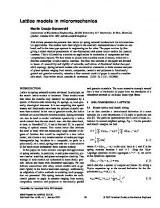
two-layer (nearest and second neighbor) particle interaction scheme, we see that the modeling crack path matches well with the experimental data (Figure 9(c)). Figure 10(a, b) exhibit a fairly good comparison of the HLPM simulation results with the according experimental observations in terms of load-energy vs. time. Here we expect that employment of α − β model may be another possible approach for eliminating a mesh effect. We will report the result to this study in our future papers.
6. Conclusions This paper proposes a hybrid lattice particle modeling (HLPM) approach for simulation of dynamic fracture phenomena in homogeneous and heterogeneous materials at macroscales with a various Poisson ratio extent. It is concerned with the mathematical derivations of employing elastic interaction formula between contiguous particles in 2D lattice networks accounting for different manners of linkage and different shapes of lattice. Then the according lattice techniques are transferred into the conventional particle modeling (PM). Consequently, a HLPM is born. All the derivations follow the equivalence of strain energy stored in a unit cell with its associated continuum structure in the case of in-plane elasticity. In this paper, axial ( α ) and combined axial-angular ( α − β ) models are accounted for together with considering triangular or rectangular lattice. Through the study, a better understanding of the suitability of different lattice models is attained to adapt to various material properties and loading conditions. Consequently, equipped with these lattice derivations, HLPM can be extended to a wider spectrum of applications in dealing with different Poisson ratios of materials at a continuum level with Poisson ratios ranging from (-1,1), no longer merely limited to 1/3 due to the application of an α -model in a 2D equilateral triangular lattice. Meanwhile, a new particle interaction scheme (i.e., nearest and second neighbor particle interaction) is proposed in a triangular lattice. The adoption of this new particle linkage mechanism successfully eliminates a bias related to the lattice geometry in use. Overall, we have found the following results from the derivations of different considerations: For α -models: (i) Nearest neighboring particle interaction:
17
(a) In a uniform triangular lattice: Poisson ratio is γ = 1 / 3 ; effective axial spring constant is α = 3E . E is the Young’s modulus. (b) In a uniform rectangular lattice considering axial-diagonal particles: Poisson ratio is γ = 1 / 3 ; effective axial and diagonal spring constants are
α I = 3E / 2, α II = 3E / 8 . (ii) Two-layer (nearest and second) neighboring particle interaction in a uniform triangular lattice: Poisson ratio is γ = 1 / 3 ; effective spring constants for the nearest and second neighboring particles are:
α I = 3E /[2(1 + 3k )], α II = 3Ek /[2(1 + 3k )] , where k is the ratio of the two spring constants. For α − β - models: (i) Nearest neighboring particle interaction: (a) In a uniform triangular lattice: Poisson ratio range is − 1 < γ ≤ 1 / 3 ; effective axial and angular spring constants are α = 2 3E /[3(1 − γ )] , β = 2 3 (1 − 3γ ) El 2 /[9(1 − γ 2 )] , where l is the half-length of the grid spacing. (b) In a uniform rectangular lattice considering axial particles: Poisson ratio γ = 0.0 ; effective axial and angular spring constants are
α = 2 E , β = El 2 / 2 . (c) In a uniform rectangular lattice considering axial-diagonal particles: Poisson ratio − 1 < γ ≤ 1 / 3 ; effective axial and angular spring constants are
α I = 2 E /(1 + γ ), α II = Eγ /(1 − γ 2 ), β = (1 − 3γ ) El 2 /[2(1 − γ 2 )] . (ii) Two-layer (nearest and second) neighboring particle interaction in a uniform triangular lattice: angular spring is invalid for a realistic model.
We finally transfer a two-layer neighboring particle interaction scheme into the PM model to simulate fracture pattern of a polymeric material (nylon-6,6) due to the
18
impact of a rigid indenter. This treatment is found an efficient approach to eliminate a mesh bias effect in the direction of crack propagation. Our future work will focus on implementing all the schemes mentioned above into PM. Calibrations of HLPM by aid of experimental data are also required.
Acknowledgement The authors would like to acknowledge the support received from the Department of Civil Engineering at the University of Mississippi, and funding received under a subcontract from the Department of Homeland Security-sponsored Southeast Region Research Initiative (SERRI) at the Department of Energy's Oak Ridge National Laboratory. We specially thank Swasti Gupta for his experimental data on nylon-6,6 impact test. The accomplishment of this paper is also greatly beneficial from the discussions with Professor M. Ostoja-Starzewski.
19
References
1. Greenspan, D., Computer-Oriented Mathematical Physics, University of Texas at Arlington, Pergamon Press, 1981. 2. Wang, G. and Ostoja-Starzewski, M., Particle modeling of dynamic fragmentation – I: theoretical considerations, Computational Materials Science, 2005, 33, 429442. 3. Wang, G., Particle modeling of dynamic fragmentation, Ph.D. Dissertation, 2005, McGill University. 4. Wang, G., Ostoja-Starzewski, M. and Radziszewski, P., Particle modeling of comminution, 20th Canadian Congress of Applied Mechanics, May 30th to June 2nd, Montreal, Canada, 2005, 149-150. 5. Wang, G., Ostoja-Starzewski, M., Radziszewski, P. and Ourriban, M., Particle modeling of dynamic fragmentation – II: fracture in single- and multi-phase materials, Computational Materials Science, 2006, 35, 116-133. 6. Ostoja-Starzewski, M. and Wang, G., Particle Modeling of Random Crack Patterns in Epoxy Plates, Probabilistic Engineering Mechanics, 2006, 21, 267275. 7. Wang, G., Radziszewski, P. and Ouellet, J., Particle modeling simulation of thermal effects on ore breakage, Computational Materials Science, 2008 (in press). 8. Greenspan, D., Supercomputer simulation of cracks and fractures by quasimolecular Dynamics, J. Phys. Chem. Solids, 1989, 50(12), 1245-1249. 9. D. Greenspan, Particle Modeling, Birkhäuser Publishing, 1997. 10. Greenspan, D., New approaches and new applications for computer simulation of N-body problems, Acta Applicandae Mathematicae, 2002, 71, 279-313.
11. Hrennikoff, A., Solution of problems of elasticity by the frame-work method, ASME, J. Appl. Mech., 1941, 8, A619-A715.
12. Askar, A., Lattice dynamical Foundations of continuum theories, World Scientific, Singapore, 1985.
20
13. Noor, A.K., Continuum modeling for repetitive lattice structures, Appl. Mech. Rev., 1988, 41(7), 285-296.
14. Ostoja-Starzewski, M., Lattice models in micromechanics, Appl. Mech. Rev. , 2002, 55(1), 35-60. 15. Grah, M., Alzebdeh, K., Sheng, P.Y., Vaudin, M.D., Bowman, K.J. and OstojaStarzewski, M., Brittle intergranular failure in 2D microstructures: experiments and simulations, Acta Mater., 1996, 44(10), 4003-4018. 16. Keating, P.N., Effect of the invariance requirements on the elastic moduli of a sheet containing circular holes, J. Mech. Phys. Solids, 1966, 40, 1031-1051. 17. Synder, K.A., Garboczi, E.J. and Day, A.R., The elastic moduli of simple twodimensional composites: computer simulation and effective medium theory, J. Mech. Phys. Solids, 1992, 72, 5948-5955.
18. Ostoja-Starzewski, M., Random field models of heterogeneous materials, Int. J. Solids Struct., 1998, 35(19), 2429-2455.
19. Bardenhagen, S. and Triantafyllidis, N., Derivation of higher order gradient continuum theories in 2D, 3D non-linear elasticity from periodic lattice models, J. Mech. Solids, 1994, 42, 111-139.
20. Chen, J.Y., Huang, Y. and M. Ortiz, Fracture analysis of cellular materials: A strain gradient model, J. Mech. Phys. Solids, 1998, 46, 789-828. 21. Holnicki-Szulc, J. & Rogula, D., Non-local, continuum models of large engineering structures, Arch. Mech., 1979a, 31(6), 793-802. 22. Synder, K.A., Garboczi, E.J., and Day, A.R., The elastic moduli of simple twodimensional composites: computer simulation and effective medium theory, J. Mech. Phys. Solids, 1992, 72, 5948-5955.
21
Figure Captions
Fig. 1 A triangular lattice with hexagonal unit cell for α model, considering nearest neighboring particle interactions. Fig. 2 Two structures for α model, I and II, resulting in a lattice with nearest neighbor and second neighbor particle interactions in central directions. Fig. 3 A rectangular lattice with rectangular unit cell for α model, considering both axial and diagonal particles. Fig. 4 A rectangular lattice with considering angular interactions. Fig. 5 A triangular lattice with hexagonal unit cell for α − β model, considering nearest neighboring particle interactions. Fig. 6 A Rectangular lattice for α − β model, without considering diagonal particles. Figure 7 A triangular lattice with hexagonal unit cell for α1 − α 2 − α 3 model, considering nearest neighbor particle interactions; after Snyder et al [22]. Fig. 8 Example of mesh effect by lattice model: compression simulation. Fig. 9 Simulation of fracture pattern of a polymeric material (nylon-6,6) due to the impact of a rigid indenter (a) experiment; (b) PM accounting for nearest particles; and (c) PM accounting for two-layer of particles. Figure 10 Profile of load and energy of a polymeric material (nylon-6,6) due to the impact of a rigid indenter (a) experiment; and (b) PM accounting for two-layer of particles.
22
Figure 1 A triangular lattice with hexagonal unit cell for α model, considering nearest neighbor particle interactions.
Figure 2 Two structures for α model, I and II, resulting in a lattice with nearest neighbor and second neighbor particle interactions in central directions [21].
23
Figure 3 A rectangular lattice with rectangular unit cell for α model, considering both axial and diagonal particles.
Figure 4 A rectangular lattice with considering angular interactions.
24
Figure 5 A triangular lattice with hexagonal unit cell for α − β model, considering nearest neighboring particle interactions.
Figure 6 A Rectangular lattice for α − β model, without considering diagonal particles.
25
Figure 7 A triangular lattice with hexagonal unit cell for α1 − α 2 − α 3 model, considering nearest neighbor particle interactions; after Snyder et al [22].
26
Figure 8 Example of mesh effect by lattice model: compression simulation (red line indicates crack path).
(a)
(b)
(c)
Figure 9 Fracture pattern of a polymeric material (nylon-6,6) due to the impact of a rigid indenter (a) experiment; (b) PM accounting for nearest particles; and (c) PM accounting for two-layer of particles.
27
(a)
(b) Figure 10 Profile of load and energy of a polymeric material (nylon-6,6) due to the impact of a rigid indenter (a) experiment; and (b) PM accounting for two-layer of particles.
28