Explore and Return: Experimental Validation of Real-Time Concurrent ...

Explore and Return: Experimental Validation of Real-Time Concurrent Mapping and Localization P. Newman J. Leonard, J. D. Tard´os, J. Neira Abstract— This paper describes a real-time implementation of feature-based concurrent mapping and localization (CML) running on a mobile robot in a dynamic indoor environment. Novel characteristics of this work include: (1) a hierarchical representation of uncertain geometric relationships that extends the SPMap framework, (2) use of robust statistics to perform extraction of line segments from laser data in real-time, and (3) the integration of CML with a “roadmap” path planning method for autonomous trajectory execution. These innovations are combined to demonstrate the ability for a mobile robot to autonomously return back to its starting position within a few centimeters of precision, despite the presence of numerous people walking through the environment.

I. Introduction Simply put, concurrent mapping and localization (CML) is the task of having a robot autonomously build a map of an unknown environment while at the same time using that map to determine its position. While there have been numerous published papers on the problem of CML in the past few years, there have been only a limited number of implementations of CML that have been operated in real-time. To our knowledge, none of these implementations (with the possible exception of Thrun [1]) have used CML in realtime to actually control the motion of the robot. This paper describes a novel, real-time implementation of CML running on a mobile robot in a dynamic indoor environment. The CML algorithm is actively used to navigate the robot. The precision and robustness of the CML process is illustrated by having a B21 mobile robot start exploring a busy hallway at MIT from a position marked with small coins on the floor. After a substantial interval the robot was commanded to return under autonomous control to its starting point. Despite P. Newman and J. Leonard are at the Department of Ocean Engineering at MIT, USA. J. Neira and J. Tardos are with the Departamento de Inform´ atica e Ingenier´ıa de Sistemas of the Universidad de Zaragoza, Spain. email: {pnewman,jleonard}@mit.edu {jneira,tardos}@posta.unizar.es.

the difficulties of map building in dynamic environments the robot stopped within 2cm of the marker dimes. The system described in this paper is entirely operating system independent. This fact coupled with the generality of the underlying mathematics and software architecture allows rapid deployment on new vehicles with various sensor configurations, operating systems and geometries. For example the software was installed and ran real-time CML on a Labmate at the University of Zaragoza, Spain in an afternoon. The union of these two demonstrations makes an important point. CML is reaching the point of maturity at which it can be considered to be an important piece of the automation engineer’s toolbox. It is possible to use CML to perform useful tasks – this paper demonstrates its use for autonomous homing. The method does not need to be hand-crafted to work on specific vehicles. II. Modeling Uncertainty The importance of the choice made in the representation of the robot’s environment cannot be under-stated. The shape and characteristics of the ensuing CML algorithm are highly dependent on this fundamental decision. To date the spectrum of representations is large, ranging from none at all [2] through grid based approaches [3] to probabilistic approaches. The later class have had the greatest success at achieving CML and can be further classified into feature based CML [4], [5], [6], [7] and data-based estimation [1]. In this paper we adopt a feature based approach. In general proprioceptive sensor data is processed to estimate parameterized geometric representations of real world entities such as walls, corners or more complex compound objects. The entire environment is described by parameterizing 2D transformations between geometric entities. For example a robot can be described by the transformation from some arbitrary reference

f

World Origin

Local Origin

Local Origin

X s,e

e

s

Robot

Sensor

Observation

Feature

Feature

Sensor

Robot

Feature

Observation

X r,s

r

Sensor

Observation

Feature

Observation

X w,f

Fig. 1. The world as a tree of transformations

w

X w,r

Fig. 2. A loop of transformations.

frame to a common reference point (CRP) on the robot. If the robot possesses sensors then these are described as a transformation from the robot’s CRP to their own centers. Similarly, the observations that a sensor makes of a real life landmark can be expressed as a transformation from sensor to perceived entity. Sequential combination of these transformations allows any one modelled component to be expressed in the coordinate frame of any other. Writing the transformation from frame i to frame j as xi,j we define the composition operator such that xi,j = xi,[·] ⊕ x[·],j

(1)

The inverse composition operator is also defined such that xi,j = ªxj,i

(2)

It is useful to visualize the structure of the model and the and relationships between its elements as a tree of transformations as shown in Figure 1. By sequential application of the composition operators it is possible to express any entity j in the coordinate frame of entity i by traversing the tree from entity i to entity j. Traversal down the tree towards leaves requires compound application of the composition operator ⊕ whereas traversal up the tree towards the root requires compound composition with the inverse transformation between nodes. Using a tree representation the exploration of new environments and discovery of new features

results in tree growth while removal of erroneous or unwanted features becomes a task of tree pruning. In the case of CML geometric entities not only have position but also an associated uncertainty. The transformation of uncertainties between coordinate frames is a well-known process in robotics [7] and is accomplished by evaluating the Jacobians of the composition operators. The system discussed in this paper utilizes the SPMap method of Castellanos et al. [8], which places this concept into a compact and succinct framework. The SPMap allows for the easy manipulation of different feature types, such as lines, points, and planes, with the same set of update equations. The method is best understood with reference to Figure 2. Consider the transformation xf ,e where the observation e is with respect to feature f ’s coordinate frame. If the measurement truly is an observation of this feature then xf ,e must be zero. Using the composition operators this can be expressed as 0 = Bf ,e [ªxw,f ⊕ xw,r ⊕ xr,s ⊕ xs,e ]

(3)

where Bf ,e is a row selection matrix that selects the relevant coordinates. With reference to Figure 2 where a line segment observation is being matched to a line feature only the lateral and orientation · ¸parameters are relevant and so Bf ,e = 0 1 0 . Castellanos et al. [8] demonstrate how 0 0 1 3 can be differentiated to produce a single set of

observation equations for use in an error state extended Kalman filter regardless of feature and observation type. Irrespective of the use of the SPMap (indeed the system can be set to use conventional feature based representations [5]) at the heart of the system lies an extended Kalman filter (EKF). The ˆ (i|j) EKF estimates at time i the state vector x and an associated covariance matrix P(i|j) given all observations up to time j. The state vector is the augmentation of the estimated vehicle state ˆ v (i|j) and N feature states p ˆ 1 ..N (i|j). x £ ˆ v (i|j)T ˆ (i|j) = x x

ˆ 1 (i|j)T · · · p

ˆ N (i|j)T p

¤T

(4)

At time k an observation z(k) of a feature becomes available. The observation is stochastically gated [9] with all existing features in the state vector in order to associate it with a particular feature. If successful, the observation is used to update the entire state vector using the standard CML Kalman equations to produce a new estiˆ (i|j) and P(i|j). mates x A major component of CML is the discovery of new features and so we expect to not be able to associate z(k) to any feature on a frequent basis. ˆ N +1 (k|k) is added to In this case a new feature p the state vector and representation tree such that ˆ N +1 (k|k) = g(ˆ p xv (k − 1|k − 1), z(k))

(5)

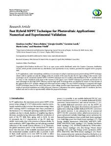
. The correlations of this new feature are also calculated and inserted into P (k|k) as originally described in [4]. In many scenarios, one with range only observations for example, it is not possible to initialize a new feature from a single observation. In this case the delayed decision framework described in [10] is invoked which allows for consistent multi-vantage point initialization of new features. Although implemented in the discussed system the experiments described use a laser scanner to produce line-segment observations which carry enough information to initialize new features. III. Implementation This section discusses some of the architectural and systems level issues involved in the development of the CML software discussed in this paper – the CMLKernel. The broad architecture of the software discussed in this section and its relationship to the physical world and client applications is shown in Figure 3. The tree representation of geometric enti-

ties, together with the unifying observation equations of the SPMap method, provide strong motivation for adopting an object oriented programming paradigm – one in which all physical entities are modeled as specializations of a fundamental object providing tree traversal, coordinate and uncertainty transformation functionality. The CMLKernel was implemented in vanilla C++ making significant use of the standard template library. Data is fed into the Kernel as ASCII sensor data strings. Similarly estimates of features and vehicle location can be retrieved in string ASCII string format. In this manner the CMLKernel can be viewed as a stand-alone navigation sensor requiring only serial port or TCP/IP connections hence avoiding tiresome software integration problems and facilitating rapid deployment. Accompanying the CMLKernel are two distinct components. Firstly, there is a hardware abstraction layer that provides an interface to the mechatronics of the host vehicle. This software provides clearly defined areas in which vehicle/sensor dependent code must be written to allow control of the vehicle and gathering of sensor data. The advantages of this abstraction layer were made evident during the deployment at the University of Zaragoza. In addition to declaring the new vehicle geometry, only the mapping from generic motion commands to the Labmate’s actuation interface and raw sensor data to string format needed to be written – a task that was swiftly accomplished. Secondly, a platform independent Berkeley socket-based communications system binds any number of vehicles, control and logging applications (including the CMLKernel) into a collaborating whole. This software, based on commonly found API, offers remarkable flexibility in configuration for example the hardware abstraction layer can be running on a vehicle running RT Linux while the CMLKernel itself is running on an NT machine connected via radio ethernet. Although a complex piece of software the CMLKernel can be understood as having a few distinct components. Input management It is not assumed that sensor data arrives in a time ordered fashion. For example on the B21 laser data arrives with a 0.7 second lag whereas the odometry is almost instantaneous. The input stage acts as a time-based priority queue that guarantees synchronous input into the rest of the kernel. Another crucial role of this stage is load monitoring of the system. If the average CPU load µ, 0 < µ < 1.0 exceeds a

Clients

Communications and Visualistion Layer

Stochastic Mapping and Localization

Data to Observations

Data Association

Robust Laser Segmentation Path Planning Sonar Clustering

CML Kernel

Feature Management

EKF

Communications and Hardware Abstraction Layer

Robot

Robot Control

Vehicle Dependent

IO Management

Fig. 3. An architecture for real-time CML

configurable threshold τ then a fraction λ of nonodometry input data is removed from the input stream. The number λ is the output if a IIR filter λt = α(µ−τ )+(1−α)λt−1 where α is the filter gain and is typically set to 0.99. This simple action ensures that an unforeseen explosion in the number of features and hence computation time required to iterate the filter will not render the system unresponsive to control commands because of CPU overloading leading to dangerous behavior. Observation Creation This stage converts raw sensor data into observations. This may involve the extraction of segments from laser scans or the utilization of delayed decision making [10] to combine sonar data measurements from multiple vantage points. Data Association This stage tries to associate observations with existing features or if no association is found potentially create new features. This is the most costly of the stages in terms of computation time. The process is split into three distinct stages. Firstly an appeal is made to the sensor physics - a decision is made on whether it is physically possible for the sensor be observing the hypothesized feature. For example the feature may be out of range of a laser scanner or in the case of sonar sensors at too great an angle of incidence to provide an acoustic return. Secondly a crude non

stochastic gate is applied. In one guise this step may prevent a segment observation being associated with a line feature with which it is co-linear but not intersecting - for example two sides of a door frame. See Section III-B for more discussion on this. Finally a chi-squared test on the innovation – the difference between predicted and actual observation – is performed. Only if all three tests pass does the observation become associated with the hypothesized feature. It is possible that the observation can be associated with more than one feature, in which case the observation is marked as ambiguous and not used in any further processing. Recent work has augmented the CMLKernel with the Joint Compatibility Test [11] which allows the resolution of the ambiguity resulting from multiple associations of an observation. Update Here new, associated observations are fused with prior estimates within the EKF. If no associated observations are available then a predict only cycle occurs with the odometry data being used as a control input into the vehicle model. Output management Finally ASCII representations of the state estimates are made and stored for retrieval by a third-party when requested. A. Feature Extraction Although the CMLKernel is capable of processing all kinds of proprioceptive sensor data, the results given in this paper are from running the kernel with odometry and laser data. This section briefly describes the process by which line segments are extracted from individual laser scans. The details of the derivations and calculations of the numeric values for the parameters discussed can be found in [12]. At the heart of the process lies a technique readily found in the robust statistics literature which has many parallels to the RANSAC method frequently used in the computer vision domain [12]. The method employed is a least median consensus technique that tries to find a line with the least median squared error between it and points in a roughly linear subset of the scan. The first phase is a classical split and merge algorithm [13] that produces clusters of scan points that are approximately linear. A least medians estimator is then applied to each of these clusters in turn. For a given expected outlier ratio, cluster size and required confidence interval, it is possible to calculate the number, θ, of randomly chosen pairs of points from which to generate a line hypothesis. For each hypothesis H1···θ the median ϑHi of the

j squared orthogonal distance δH from the line to i the each point j in the remaining cloud of points is calculated. The hypothesis Hmin with the smallest median distance is then taken to be the best linear fit. Based on ϑHmin a threshold distance τHmin is calculated which allows the j th point in the cluster to be classed as an outlier and removed from j > τHmin . An eigenvalue dethe cluster if δH min composition (or total least squares) is then carried out on the remaining points to determine the best fit and covariance of the line with respect to the inliers alone. The resulting line and its associated covariance is then passed as an observation to the update stage of the CMLKernel. By specifying a minimum acceptable segment observation length this method can be made to be remarkably robust in noisy environments, as will be shown in the results section. A clear benefit of using line segment observations is the large amount of angular information they convey. An observation of a wall resulting in a segment observation of perhaps 1.5 m has very little angular error with respect to the robot frame of reference. This is of great consequence given that it is well understood that large angular errors in EKF based CML algorithms can lead to instability and filter divergence.

B. Optional Browsing for Structure As a background task the CMLKernel can optionally be configured to browse its internal tree of features and look for “anthropomorphic” structure such as parallelism or orthogonality between line type features – common phenomena in indoor environments. Randomly pairs of features are chosen and hypotheses generated in the form of Equation 3 under the assumption that they are co-linear, parallel or orthogonal. If a hypothesis passes a chi-squared significance test [9], this hypothesis is converted to an artificial observation with a configurable covariance or uncertainty (typically large). The effect of this process is that lines that are almost orthogonal tend to become orthogonal, with similar effects for parallel lines. Clearly invoking this process while in a pathological environment such as a large circular hall with gently curving but “almost” straight walls would cause this method to fail. It should also be stated that if this option is used, a priori relative [7] information is being added to the map and hence the correlations between features increase more rapidly than would be the case in normal circumstances. However, at

no point is artificial absolute information added and thus the limiting uncertainty in the absolute feature locations remains unchanged. C. Planning a Path Home An important component of a successful CML demonstration is a the ability of a robot to use the feature based map to perform some useful action. In this section we describe a method by which using a stochastic map built by the CMLKernel the robot autonomously returned to its initial starting position with less than one inch of error. As the vehicle explores its environment the CMLKernel occasionally drops “virtual free-space markers” at its current estimated position. These markers form a connected graph of regions of free space [14]. Markers are only dropped when the un-occluded distance to the nearest previously dropped marker is greater than some arbitrary value (in our experiments 1-2m). The task of navigating to an arbitrary point then becomes one of driving to the nearest virtual marker and then following the free space graph to get within an acceptable distance from the desired location. The robot must then leave the “free space highway” and drive in a straight line to the goal position. The first free space marker is dropped at the initial robot position. The task of returning home is then reduced to one of traversing the free space graph until the root node is reached. Each marker contains a “score” that defines the minimum number of markers from itself that need to be traversed before the origin or first dropped marker is reached. In this manner at each node in the graph a decision can be made as to which marker to head towards next. A simple control algorithm is used to execute the transitions to free space markers. First the robot rotates in-situ until its forward axis points directly at the target marker xt . It then translates the required distance to the goal position. While undertaking this motion the CML process continually updates the location of the robot as and when sensor data arrives. This allows dynamic feedback to correct the vehicle trajectory in real time as a function of the stochastic map. IV. Experimental Results This section describes a substantive deployment of CML in a moderately sized and highly dynamic environment. The experiment was undertaken in a large hallway at MIT during a busy time of the day. A commercially available B21 mobile robot

Fig. 5. The experiment scene

Fig. 4. Re-observing an existing feature

fitted with a radio ethernet ran the hardware abstraction layer under Linux and relayed data via the comms layer to a laptop running the CMLKernel and a 3D OpenGL renderer under NT 1 . The only sensors used were a SICK laser scanner and wheel encoders mounted on the vehicle. The floor surface was a combination of sandstone tiles and carpet mats providing alternatively high and low wheel slippage. The exploration stage was manually controlled although it should be emphasized that this was done without visual contact with the vehicle. The output of the CMLKernel was rendered in 3D and used as a real-time visualization tool of the robot’s workspace. This enabled the remote operator to “visit” previously un-explored areas while simultaneously building an accurate geometric representation of the environment. This in itself is a useful application of CML; nevertheless, future experiments will implement an autonomous explore function as well as the existing autonomous return. To illustrate the accuracy of the CML algorithm the starting position of the robot was marked with four ten-cent coins; the robot then explored its environment and when commanded used the resulting map to return to its initial position and park itself on top of the coins with less than 2cm of error. The duration of the experiment was 1 It

is important to note that the kernel could just as well have been run on the B21 itself but running a local version offers debugging advantages.

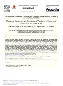
a little over 20 minutes with just over 6MB of data processed. The total distance travelled was well in excess of 100m. Videos of various stages of the experiment can be found in various formats at http://oe.mit.edu/~pnewman. Figure 5 shows the environment in which the experiment occurred. The main entrance hall to the MIT campus was undergoing renovation during which large wood-clad pillars had been erected throughout the hallway, yielding an interesting, landmark-rich and densely populated area. Figures 4 and 6 show rendered views of the estimated map during the exploration phase of the experiment. In Figure 4 the robot can be seen to be applying a line segment observation of an existing feature. In contrast Figure 6 shows an observation initializing a new feature just after the robot has turned a corner. The dotted lines parallel to the walls are representations of lateral uncertainty in that wall feature2 . The vehicle was started with an initial uncertainty of 0.35 m and as shown in [15] all features will inherit this uncertainty as a limiting lower bound in their own uncertainty. The 1σ uncertainty of the vehicle location is shown as a dotted ellipse around the base of the vehicle. Figure 9 shows an OpenGL view of the estimated map towards the end of the experiment when the robot is executing its homing algorithm. 2 One benefit of the SPMap is that the states estimated for line are precisely the lateral and angular errors of the wall in its local coordinate frame, hence drawing the uncertainty is a trivial matter.

Fig. 7. The starting position

Fig. 8. The robot position after the completion of the homing leg of the mission Fig. 6. Creating a new feature in the foreground following a rotation

goal seeking tolerance ² is reduced to 1cm. The CMLKernel spent about thirty seconds commanding small adjustments to the location and pose of the robot before declaring that the vehicle had indeed arrived back at its starting location. Figures 7 and 8 show the starting and finishing positions with respect to the coin markers. As can be seen in these figures the vehicle returned to within an inch of the starting location. Readers are invited to view videos of this experiment and others including navigation in a populated museum at http://oe.mit.edu/~pnewman. V. Future work Fig. 9. A plan view of the CML map at the end of the experiment. The approximate size of the environment was a 20m by 15m rectangle.

The circles on the ground mark the free space markers that were dropped during the exploration phase of the experiment. The homing command was given when the robot was at the far corner of the hallway. Using the output of the CMLKernel, the robot set the goal marker to be the closest way point. When the algorithm deduces that the vehicle is within an acceptable tolerance ² of the present goal marker it sets the goal way-point to be the closest marker that has a score less than the present goal marker as described in Section III-C. This then proceeds until the goal marker is the origin or initial robot position. At this point the

The CMLKernel is part of an ongoing program of CML research at the MIT Department of Ocean Engineering. The software is currently being deployed in the sub-sea domain on autonomous underwater vehicles (AUVs) using inputs from beacon-based long baseline acoustic systems with no prior knowledge of beacon locations. The extension to multi-map navigation is an important avenue to pursue, to enable real-time CML in large-scale environments [16], [17], and is currently underway. CML with multiple submaps can be viewed as a depth-wise expansion of the representation tree. Vehicles belong to submaps which in turn belong to the world frame. Both the Joint Compatibility Test presented in [11] and the delayed decision making framework described in [10] have been implemented in the

CMLKernel. However the fusion of these methodologies into a single approach may yield a robust and powerful spatio-temporal data association and feature creation capability. As has always been the case with EKF-based CML methods the algorithm is ill affected by the effects of linearization in the presence of large angular error. This situation is most likely to occur during or just after maneuvers containing a large rotational components or when operating in a large single map (rather tan using multiple small maps). Detecting and coping with such scenarios and actively controlling perception to minimize angular error may significantly improve robustness and facilitate performing CML around large loops. Acknowledgements This research has been funded in part by NSF Career Award BES-9733040, the MIT Sea Grant College Program under grant NA86RG0074 (project RCM-3), and Ministerio de Educaci´ on y Cultura of Spain, grant PR2000-0104, and by the Spain-US Commission for Educational and Scientific Exchange (Fulbright), grant 20079.

References [1]

S. Thrun, “An online mapping algorithm for teams of mobile robots,” Int. J. Robotics Research, vol. 20, no. 5, pp. 335–363, May 2001. [2] R. A. Brooks, “Intelligence without representation,” Artificial Intelligence, vol. 47, pp. 139–159, 1991. [3] A. Elfes, “Sonar-based real-world mapping and navigation,” IEEE Journal of Robotics and Automation, vol. RA-3, no. 3, pp. 249–265, June 1987. [4] R. Smith, M. Self, and P. Cheeseman, “A stochastic map for uncertain spatial relationships,” in 4th International Symposium on Robotics Research. MIT Press, 1987. [5] J. J. Leonard and H. F. Durrant-Whyte, Directed Sonar Sensing for Mobile Robot Navigation, Boston: Kluwer Academic Publishers, 1992. [6] J. A. Castellanos, J. D. Tardos, and G. Schmidt, “Building a global map of the environment of a mobile robot: The importance of correlations,” in Proc. IEEE Int. Conf. Robotics and Automation, 1997, pp. 1053–1059. [7] P. M. Newman, On the structure and solution of the simultaneous localization and mapping problem, Ph.D. thesis, University of Sydney, 1999. [8] J. A. Castellanos, J. M. M. Montiel, J. Neira, and J. D. Tardos, “The SPmap: A probabilistic framework for simultaneous localization and map building,” IEEE Trans. Robotics and Automation, vol. 15, no. 5, pp. 948–952, 1999. [9] Y. Bar-Shalom and T. E. Fortmann, Tracking and Data Association, Academic Press, 1988. [10] J. J. Leonard and R. Rikoski, “Incorporation of delayed decision making into stochastic mapping,” in Experimental Robotics VII, D. Rus and S. Singh, Eds., Lecture Notes in Control and Information Sciences. Springer-Verlag, 2001. [11] J. Neira and J.D. Tard´ os, “Data association in stochastic mapping using the joint compatibility test,” IEEE

[12] [13] [14] [15]

[16]

[17]

Trans. on Robotics and Automation, vol. 17, no. 6, pp. 890–897, 2001. R. I. Hartley and A. Zisserman, Multiple View Geometry in Computer Vision, Cambridge University Press, ISBN: 0521623049, 2001. T. Pavlidis, Algorithms for Graphics and Image Processing, Computer Science Press, 1982. J-C. Latombe, Robot Motion Planning, Boston: Kluwer Academic Publishers, 1991. M. W. M. G. Dissanayake, P. Newman, H. F. DurrantWhyte, S. Clark, and M. Csorba, “A solution to the simultaneous localization and map building (slam) problem,” IEEE Transactions on Robotic and Automation, vol. 17, no. 3, pp. 229–241, June 2001. J. J. Leonard and H. J. S. Feder, “A computationally efficient method for large-scale concurrent mapping and localization,” in Robotics Research: The Ninth International Symposium, D Koditschek and J. Hollerbach, Eds., Snowbird, Utah, 2000, pp. 169– 176, Springer Verlag. J. Guivant and E. Nebot, “Optimization of the simultaneous localization and map building algorithm for real time implementation,” IEEE Transactions on Robotic and Automation, vol. 17, no. 3, pp. 242–257, June 2001.