AbstractâInformation extraction from text databases is a useful paradigm to populate relational tables and unlock the considerable value hidden in plain-text ...
Exploring a Few Good Tuples From Text Databases Alpa Jain1 , Divesh Srivastava2 1
Columbia University, 2 AT&T Labs-Research
Abstract— Information extraction from text databases is a max is the maximum number of terms in an extraction pattern useful paradigm to populate relational tables and unlock the and x is the number of word transformations for a tuple context considerable value hidden in plain-text documents. However, to match the pattern, then the confidence score is computed as information extraction can be expensive, due to various complex x text processing steps necessary in uncovering the hidden data. 1 − max (x ≤ max). Given a text snippet, “A Cholera outbreak There are a large number of text databases available, and not is sweeping throughout Sudan as of ...,” and max = 4, the every text database is necessarily relevant to every relation. extraction system generates the tuple hCholera, Sudani with Hence, it is important to be able to quickly explore the utility a score of 1.0 (x = 0). On the other hand, for a text snippet, of running an extractor for a specific relation over a given text “... checking for Measles is America’s way of avoiding ...,” the database before carrying out the expensive extraction task. In this paper, we present a novel exploration methodology of finding extraction system generates the tuple hMeasles, Americai with a few good tuples for a relation that can be extracted from a a lower confidence score of 0.25 (x = 3). � database which allows for judging the relevance of the database A tuple may also be associated with multiple scores: facts for the relation. Specifically, we propose the notion of a good(k, `) are often repeated across text documents and this redundancy query as one that can return any k tuples for a relation among the top-` fraction of tuples ranked by their aggregated confidence can be used to further boost the confidence score of a tuple [9]. scores, provided by the extractor; if these tuples have high Example 1.2: (continued). Using the same extraction sysscores, the database can be determined as relevant to the relation. tem in Example 1.1 to process another document in the We formalize the access model for information extraction, and investigate efficient query processing algorithms for good(k, `) collection that contains the text snippet, “A cholera outbreak queries, which do not rely on any prior knowledge about the sweeping throughout Sudan resulted in ...” will result in extraction task or the database. We demonstrate the viability of extracting the same tuple in Example 1.1 but now with a our algorithms using a detailed experimental study with real text score of 0.75 (x = 1). � databases.
I. I NTRODUCTION Oftentimes, collections of text documents such as newspaper articles, emails, web documents, etc. contain large amounts of structured information. For instance, news articles may contain information regarding disease outbreaks which may be put together using the relation DiseaseOutbreakhDisease, Locationi. To access these relations, we must first process documents using an appropriate information extraction system. Examples of reallife extraction systems include Avatar1 , DBLife2 , DIPRE [3], KnowItAll [10], Rapier [5], Snowball [2]. These relations that are extracted from text documents differ from traditional relations in one important manner: not all tuples in the extracted relations may be valid instances of the target relation [14], [16]. To reflect the confidence in an extracted tuple, extraction systems typically assign a score along with an extracted tuple (e.g., [2], [9], [10]). Example 1.1: Consider the task of extracting information about recent disease outbreaks to generate the DiseaseOutbreak relation. We are given an extraction system, that applies the pattern ”hDiseasei outbreak is sweeping throughout hLocationi” to identify the target tuples. As a simple example of confidence score assignment, consider the case where the extraction system uses edit-distance-based similarity matching between the context of a candidate tuple and the pattern. Specifically, if 1 http://www.almaden.ibm.com/cs/projects/avatar 2 www.dblife.cs.wisc.edu
The total confidence score of a tuple is an aggregation of individual scores derived from processing different documents. We can amass available scores for tuples and rank them using an aggregate scoring function, while viewing extraction systems as “black-boxes” that take as input a document and produce tuples along with some confidence scores as illustrated in the examples above. Typically, good tuples such as hCholera, Sudani will occur multiple times [9] and thus, have their overall confidence scores boosted; on the other hand, low quality tuples such as hMeasles, Americai will be sparse and not have their scores boosted. This notion of a score per tuple provides an opportunity for ranking the extracted tuples and, in turn, allowing for a new query paradigm of exploring a few high-ranking good tuples. As a concrete example scenario for this query paradigm, in this paper, we consider the problem of exploring the potential of a text corpus for extracting tuples of a specific relation. Information extraction on a large corpus is a time-consuming process because it often requires complex text processing (e.g., part-of-speech or named-entity tagging). Before embarking on such a time-consuming process on a corpus that may or may not yield high confidence tuples, a user may want to extract a few good tuples from the corpus, allowing the user to make an informed decision about deploying an information extraction system. For instance, given the task of extracting the DiseaseOutbreak relation, a test collection that contains Sports-related documents from a newspaper archive is unlikely to generate tuples with high confidence scores. Knowing the
0
d1
d2
d3
d4
d5
d6
d7
d8
d9
d10
d11
1
t1 1.0 0 0 0 0 0 0 0 0.75 0 0.6 C nature of tuples that are among the high ranking tuples can B B C 0 0 0 0 0 0.5 0.8 0 0 0 0 B t2 C C 0.2 0 0 0.6 0 0 0 0 0 0 0 B t3 C help decide whether processing the entire corpus is desirable. B B C 0 0 0 0 0.6 0 0 0.1 0 0 0 B t4 C B C t5 0.1 0.1 0 0 0.2 0 0.6 0 0 0 0 C How can we identify a few good tuples for a relation buried B B C 0 0 0 0 0 0 0 0 0 0.3 0 B t6 C B C t7 0 0 0 0 0 0.6 0 0 0 0.7 0 C in a text database? The first solution that suggests itself is to B B C 0 0 0 0 0.3 0 0 0 0 0 0 B t8 C B C t9 0 0 0 0.2 0 0 0 0.2 0.2 0 0 C draw a random sample of tuples in the database, by processing B B C 0.05 0 0.15 0 0 0 0 0 0 0 0 B t10 C B C t11 0 0 0 0 0 0 0 0 0 0 0.05 C a random set of database documents using an appropriate B B C 0 0.9 0 0 0.9 0 0 0.9 0 0.9 0 B t12 C B C t13 0 0 0 0 0.1 0 0 0 0 0 0 C extraction system. Unfortunately, this approach leads to a B B C 0 0 0.1 0 0 0 0 0 0 0 0 B t14 C B C t15 0 0 0 0 0 0 0 0.5 0 0 0 C negatively biased view of the database: typically text databases B B C 0 0 0 0 0 0 0 0 0 0 0.7 C B t16 B C t17 0 0 0 0 0 0 0 0 0 0.4 0 C (even those that are relevant to a relation) contain a relatively B B C 0.3 0 0 0.2 0 0.3 0 0 0.4 0 0 B t18 C @ t A 0 0.5 0 0 0 0 0.5 0 0 0 0 large number of low scoring, incorrect tuples, which, in turn, 19 t20 0 0 0 0 0 0.1 0 0 0 0 0 leads to large number of low scoring tuples (false positives) in a random sample of tuples. Another solution is to derive the Fig. 1. Sample matrix of confidence scores. top-k ranking tuples of the relation based on the aggregated scores of each tuple. However, using top-k query models is “right-sized” candidate set. In summary, the contributions of undesirable since, as we will see, deriving the top-k answers in this paper are: our extraction-based scenario requires near complete processing • We formalize a new query model, i.e., good(k, `) for the of a database, for each relation. task of exploring databases for an extraction system. In this paper, we propose a novel approach to identify a few • We present two query processing algorithms for the good tuples for a relation based on returning any k tuples among good(k, `) queries, one deterministic and the other probathe top-` fraction of tuples ranked by their aggregate confidence bilistic, which do not rely on any prior knowledge of the scores. We refer to this as the good(k, `) model, and investigate extraction task or the database, making them suitable for the problem of efficiently identifying good(k, `) answers from our data exploration task. a text database. An intuitively appealing solution to process a • We evaluate the effectiveness of our algorithms using a good(k, `) query is to draw a set of k` tuples from the database detailed experimental study over a variety of real text data and return the top-k tuples among the candidate set. Such a twosets and relations. phase approach allows to focus the expensive extraction process The rest of this paper is organized as follows: Section II on only a small subset of the database. However, following this introduces and formally defines our data, access, and query approach poses several important challenges. First, we need to models. In Section III, we present an overview of our query build efficient algorithms to identify the final k answers among processing approach. In Section IV we present good(k, `) a candidate set. Second, we need to identify an appropriate size processing algorithms, which consist of a deterministic and for the candidate set, so that it contains enough answer tuples a probabilistic algorithm. In Section V we discuss how we and at the same time avoids wasteful processing of documents. pick an initial candidate set of tuples to be processed by the To identify the set of k answers from a candidate set, we proposed algorithms. We then present our experimental results propose two algorithms. Our first algorithm, E -Upper , is a in Sections VI. Section VII discusses related work. Finally, we deterministic algorithm, that adapts an existing top-k algorithm, conclude the paper in Section VIII. namely Upper [4], to our setting. The second algorithm, II. DATA , ACCESS , AND Q UERY M ODELS Slice, is a probabilistic algorithm which recursively processes documents identified through query-based access, returning We first define the data and access models which form the promising subsets of the candidate tuple set that are likely basis of our query processing scenario. We then formalize the to be in the good(k, `) answer set, while performing early good(k, `) query model and the problem we address. pruning on subsets that are unlikely to be in the answer set. This repeated triage is achieved by modeling the evolution of A. Data model The primary type of objects in our query processing ranks of tuples as a sequence of rank inversions, wherein pairs of adjacent tuples in the current rank order independently switch framework are tuples extracted from a text database D using rank positions with some probability. Within this framework, an extraction system E. Given a tuple t, we describe t as a query processing time can be reduced by trading off time with vector sv(t) = [s1 , s2 , · · · , s|D| ], where sj (0 ≤ sj ≤ 1) is the score assigned to the tuple after processing document dj answer quality, in a user-specific fashion. Identifying a “right-sized” candidate set is non-obvious (j = 1 . . . |D|). For documents that do not generate a tuple, because of the skew in the distribution of tuple occurrences. the associated score element is 0. Depending on how we choose to aggregate individual scores of Example 2.1: Consider a sample matrix of scores for tuples a tuple we may be more (or less) likely to observe a frequently across documents with documents as columns and tuples as occurring tuple at a given rank. To account for the effect of rows (see Figure 1). Each element (i, j) in the matrix represents the aggregate scoring function and the skew in the number the score for tuple ti after processing document dj . For instance, of tuple occurrences, we present a iterative method that first tuple t1 represents the tuple hCholera, Sudani from Example 1.1 learns the relevant parameters of the data using a small sample, which was extracted from two documents, denoted as d1 and and then uses the learned parameters to adaptively choose a d9 from our previous examples. Additionally, t1 also occurs
in a third document d11 with a score of 0.6. Thus, sv(t1 ) = [1.0, 0, 0, 0, 0, 0, 0, 0, 0.75, 0, 0.6]. � Given a tuple t, we derive its final score s(t) using an aggregate function. In our discussion, we consider two aggregate functions. Our first function is summation, a common choice, which computes the final score of a tuple t as the sum of the elements in the associated score vector. Specifically, |D| X s(t) = si (1) i=1
where si are the elements in sv(t). We refer to this function as sum. For instance, the final score for the tuple t1 in Figure 1 using sum is 2.35. For our second aggregate function, we view the observed occurrences of a tuple along with their confidence scores as independent events. To compute the aggregated confidence, we derive the probability of the union of these events occurring based on the Inclusion-exclusion principle. Specifically, n X X X s(t) = si ·sj − si ·sj ·sk +. . . (2) si − i=1
i,j: 1≤i β: Then, {top-β of C 0 } ⊂ {top-γ of C 0 }. This means that at least β tuples from the top-γ of C 0 are contained in the top-α of C. So, at most γ − β tuples from the top-γ of C 0 are not contained in the top-α of C. Therefore, out of the δ tuples from R0 that are contained in the top-γ of C 0 at most γ − β can not be contained in the top-α of C. Case 2: γ ≤ β: Then, {top-γ of C 0 } ⊆ {top-β of C 0 } ⊆ {top-α of C}. Hence, all δ tuples in R0 are contained in the top-α of C. We are now ready to prove Theorem 4.1. Proof: By induction on the recursion height. Base cases: (a) If a ≤ �, Slice returns R = ∅, which trivially satisfies the condition that |R| ≤ a and R contains at least a − � tuples from the top-a of C. (b) If |C| = a, Slice returns R = C, which trivially are the top-a tuples in C. Induction step: Slice picks �˜, X, and Y (see Figure 4). Let Xb and Yg denote the false positives in X and the false negatives in Y , respectively. Let R0 be the set of tuples returned by the recursion call Slice(C − X − Y, a − |X|, � − �˜). From the induction hypothesis we know that |R0 | ≤ a − |X|, and, since R = R0 ∪ X, we can conclude that |R| ≤ a. To calculate the number of tuples in R that belong to the top-a of C, we identify the following properties used in our proof: (1) |X| contains |X| − |Xb | tuples from the top-a tuples in C. (2) C 0 contains (a − |X − Xb | − |Yg |) tuples from the top-a tuples in C. (3) By the induction hypothesis, R0 contains at least a − |X| −(� − �˜) from the top-(a− |X|) tuples in C −X −Y . Applying Lemma 4.2 to C 0 , where C 0 = C − X − Y , with α = a, β = a − (|X| − |Xb |) − |Yg | (by property (2)), γ = a − |X|, and δ = a − |X| − (� − �˜) (by property (3)), we get
that the set R0 contains at least a − |X| − (� − �˜) − max [(a − |X|) − (a − (|X| − |Xb |) − |Yg |), 0] tuples that belong to the top-a of C. We further solve this to derive the total number of tuples in R0 that are in the top-a of C to be: a − |X| − (� − �˜) − max [|Yg | − |Xb |, 0] = a − (|X| − |Xb |) − (� − �˜) − max [|Yg |, |Xb |] ≥ a − (|X| − |Xb |) − (� − �˜) − �˜ (by |Yg |, |Xb | ≤ �˜) = a − (|X| − |Xb |) − � Furthermore, we know that R = R0 ∪ X. Using property (1), we can conclude that R must contain at least a−(|X|−|Xb |)− � + |X| − |Xb | = a − � tuples from top-a of C. 1) Deriving Rank-based Boundaries: We now discuss how we pick the rank-based boundaries τg and τb in order to generate the sets X and Y at each recursion. Given a candidate set C and the goal of fetching top-a tuples in C, we observe that using a rank boundary τg generates a false positive when a tuple at a rank greater than than a is observed at a rank less than τg . To compute the expected number of false positives given τg and a, we study the probability of such rank inversions taking place. Formally, we are interested in deriving the probability P rinv {j, i} that a tuple at rank j is observed at rank i where j > i after processing α · r fraction of documents, where r is the number of recursion levels so far. A rank inversion between positions j and i would, in turn, require a series of consecutive rank swaps to take place, i.e., the tuple must ”swap” ranks with all the tuples with ranks q, where j > q > i. Figure 6 illustrates the generation of a false positive for a set C of ranked tuples, with 1 being the top rank and |C| the largest possible rank. For a given a, the figure illustrates one possible choice of τg which results in a single false positive at position 3. This false positive was generated when a tuple with actual rank = a+1 swapped ranks with all other tuples with smaller ranks until it arrived at the observed rank of 3. In practice, the relation between rank swaps and a rank inversion of a specific length can be arbitrarily complex depending on the nature of the text database, the tuple score distribution, etc. To avoid relying on any apriori knowledge or sophisticated statistics, we make a simplified assumption of independence across different rank swaps. Specifically, we can derive P rinv {j, i} as: P rinv {j, i} =
i Y
P rinv {q + 1, q}
(3)
q=j
The probability of a single rank swap i.e., a tuple with actual rank j swaps ranks with a tuple with actual rank (j + 1), depends on the fraction (α · r) documents processed for the candidate tuples. Specifically, we denote the probability of a single rank swap as a function fs (β) of the fraction of documents β = (α · r) processed for the candidate tuples. Following this, the expected number of false positives when using τg as the boundary is: τg τg X X E[false positives|β, τg ] = P rinv {a+1, j}= fs (β)(a+1−j) j=1
j=1
|C|
Fig. 6.
a
τg
1
A false positive generated by a series of consecutive rank swaps.
This is a conservative upperbound on the expected number of false positives as we compute the rank inversions between the ranks τg and a + 1; tuples with ranks greater than a + 1 are less likely to switch over as false positives than the tuple at rank a + 1. To compute fs (β) given the fraction β of documents processed, we estimate the probability of a rank swap for varying values of β at runtime. Specifically, we begin with a small sample S of tuples (e.g., 5 or 10 tuples) and examine the probability of rank swap by varying the values for β. Given an aggregate function, and a β value we process β fraction of the documents associated with the tuples in S. Using the aggregate function along with the scores observed so far, we derive a ranked list of the tuples in S. To derive fs (β), we now compute the total number of rank inversions observed in this ranked list and normalize it by the maximum number of inversions possible in a sequence of size |S|. As we will see later, this step of estimating fs (β) can be “piggy-backed” with the process of deriving other parameters necessary for query processing (Section V). So far, we discussed how we derive the rank boundary τg for generating the set X. To derive the rank boundary τb , we proceed in a similar fashion after computing the expected number of false negatives for a given τb and a. 2) Choosing an Error Budget: We now discuss the issue of picking �˜, i.e., the maximum allowed false positives (or false negatives) at each recursion level. For this, we first discuss the general effect of the choice of �˜. Given two different recursion levels r1 and r2 where r2 > r1 and a �˜ value, the set X2 picked by Slice at recursion level r2 is larger than the set X1 picked at level r1 . This is mainly because at r2 , Slice would have observed and processed more documents than at r1 , thus moving closer to the actual ranking of the candidate tuples and reducing the chance of picking a false positive. This, in turn, allows Slice to pick a larger value for τg at r2 than at r1 for the same �˜ value, resulting in X2 such that |X2 | > |X1 |. This observation gives us an incentive to increase the number of recursion levels by picking a small value for �˜ during the initial levels of recursion. However, deeper recursion levels come at the cost of processing more documents as Slice processes a new fraction of documents at each level. On the other hand, given a recursion level r and two different values for the error budget �˜2 and �˜1 , where �˜2 > �˜1 , the set X2 picked by Slice using �˜2 is larger than the set X1 picked by Slice using �˜1 . This is because using �˜2 allows for more slack and enables a more aggressive approach at building X by picking a larger value for τg compared to that picked using �˜1 . While using larger values for epsilon earlier on can reduce the number of recursion levels (and thus the cost of the algorithm), we run into the risk of exhausting the error budget too soon and having to process all the remaining documents: when �˜ = 0,
Slice is not permitted any false positives or false negatives, and Slice must process all documents for each tuple in C. We studied alternative definitions for the getNextError and found the function �˜ = 2� to work well; halving the available error budget at each level ensures we use error budgets in proportion to the expected error. V. G ENERATING C ANDIDATE S ETS Our algorithms of Section IV rely on a getCandidate(k, `, δ) procedure to generate a candidate set of tuples C that, with probability at least 1−δ, contains at least k tuples from the top` fraction of the database tuples. We now present two methods to derive such a candidate set, a Naive method (Section V-A) and an Iterative method (Section V-B). A. The Naive Approach Given the goal of constructing a candidate set that contains k tuples from the top-` fraction of the tuples in the database, we begin with drawing a random sample of the tuples via S-access. Specifically, our goal is to process documents retrieved by Saccess until we have extracted k tuples from the top-` fraction. For this, we observe that the number of tuples in C that belong to the top-` fraction of the tuples in the database is a random variable VH that follows a hypergeometric distribution. Thus, P r{VH < k} =
k−1 X
Hyper (T , T · `, |C |, j )
(4)
j=0
(gi)·(D−g S−i ) . For a desired confidence (DS) (1 − δ) in the candidate set, we can draw samples C such that the probability that C contains at least k answers exceeds 1 − δ. Hence, we are looking for: where Hyper (D, S, g, i) =
min{|C| : (1 − P r{VH < k}) ≥ (1 − δ)}
(5)
In practice, though, deriving the cumulative distribution function of a hypergeometric distribution does not yield a closed-form solution. To optimize the process of selecting a candidate set we can model the sampling process using a binomial distribution. Besides simplifying the candidate set size derivation, using a binomial model provides an added benefit of not requiring the knowledge of the exact number of tuples in the database. This is particularly appealing in a data exploration setting where the total number of tuples is not known a priori. Under the binomial model, the number of tuples in C that belong to the top-` fraction of the tuples that can be extracted from the database is a random variable VB with probability of success p = ` such that: k−1 X �|C|� P r{VB < k} = · pj (1 − p)|C|−j (6) j j=0 Equation 5 gives us the size of candidate set to draw. Finally, for p ≥ 0.5 we can further use Chernoff bounds [18] to derive an upper bound on |C|. The approach outlined above assumes no skew in the data and that a set of tuples derived using S-access is an unbiased
B. The Iterative Approach In some cases, we may have a skewed database such that some tuples occur more frequently than the others. In fact, [15] showed that the extracted tuples in a database follow a long tail distribution, i.e., a power-law distribution. In this setting, it becomes important to examine the effect of the choice of the aggregate function on the rank of a frequently occurring tuple or that of a rarely occurring tuple. Specifically, we want to examine for a given function the relation between the frequency of a tuple and the fraction of the ranked tuples it belongs to. Consider the case of summation. Informally, a tuple that occurs very frequently is more likely to have a high score and thus occur towards the top of the ranked list of tuples (i.e., small values of `) than a tuple that occurs only once. Furthermore, a frequently occurring tuple is more likely to be observed in a random sample than a rarely occurring tuple. As a consequence, for small values of `, the samples drawn using S-access may contain more tuples than necessary to derive a good(k, `) answer. This, in turn, implies that we can down sample when selecting the candidate set for smaller values of ` when using summation as the aggregation function. As a contrasting example, consider the case where the scoring function is min, i.e., the final score of a tuple is the minimum score assigned to it across all documents. In this case, a rarely occurring tuple is more likely to belong towards the top of the ranked list of tuples, and this would require us to over sample when constructing the candidate set for small values of `. To account for the scoring function effect, we developed a two-step candidate generation approach. Given the goal of constructing a candidate set containing k tuples from the top-` fraction of the tuples in the database, we pick a small value s (s � k) and construct an initial candidate set that contains s tuples that belong to the top-` fraction of the tuples in the database. We generate this initial candidate set using the Naive method outlined in Section V-A. Using Q-access, we derive the matching documents for each tuple in this set, and process them to derive for each candidate tuple the actual aggregate score. To this end, we compute an adjust factor a(`). Specifically, we calculate the actual number of tuples in the initial candidate set that belong to the top-` fraction of all the tuples and divide this number by s. When using a function like sum that calls for down sampling, a(`) ≥ 1. We apply this adjust factor when constructing a candidate set for the remainder k − s tuples to be fetched. Specifically, we now target for k−s a(`) tuples instead of (k − s) tuples to generate the remainder of the candidate set. The two-step approach discussed above can naturally be extended to a fully iterative approach where we refine our
1
EU-I EU-N
0.8
Execution Cost
Execution Cost
1
random sample of the tuples in the database. In particular, it assumes that (a) each tuple occurs only once or the frequency of the tuples is uniform, and (b) the choice of the aggregate function does not affect the likelihood of observing a tuple that belongs to the top-` fraction of the tuples that can be extracted from the database. Next, we present another approach for constructing the candidate set that relaxes these assumptions.
0.6 0.4 0.2
EU-I EU-N
0.8 0.6 0.4 0.2 0
0 0.1
0.2
0.3
top-l fraction
0.4
0.5
0.1
0.2
0.3
0.4
0.5
top-l fraction
Fig. 7. Average execution cost using E -Upper for varying ` using (a) sum and (b) incl-excl.
estimate for a(`) iteratively. Using the adjust factor obtained at iteration i from si , we can decide an appropriate scaling factor when fetching the si+1 tuples in the i + 1st iteration. Interestingly, our experiments reveal that fixing the number of iterations to two (i.e., n = 2) results in candidate sets with sizes close to those we can obtain if we had perfect knowledge of the scoring function effect. VI. E XPERIMENTAL E VALUATION We now describe the settings for our experiments and report the experimental results. Information Extraction Systems: We trained Snowball [2] for two relations: HeadquartershCompany, Locationi, and ExecutiveshCompany, CEO i Data Set: We used a collection of newspaper articles from The New York Times from 1995 (NYT95) and 1996 (NYT96), and a collection of newspaper articles from The Wall Street Journal (WSJ). The NYT96 database contains 135,438 documents and we used it to train the extraction systems. To evaluate our experiments, we used a subset of 49,527 documents from NYT96, 50,269 documents from the NYT95, and 98,732 documents from the WSJ. Queries: To generate good(k, `) queries, we varied ` from 0.05 to 0.5, in steps of 0.05, and used k ranging from 20 to 200, in steps of 20. For each good(k, `) query, we report values averaged across 5 runs. Metrics: To evaluate a processing algorithm, we measure the precision and the recall of the answers generated by the algorithm for a given good(k, `) query. Given a good(k, `) query, if G is the actual set of tuples in the actual top-` fraction, and R is a set of answers, we define: |G ∩ R| |G ∩ R| P recision = ; Recall = min( , 1.0) (7) |R| k In addition to the precision and recall, we also derive the execution cost of deriving an answer using Definition 3.1. Combining query processing algorithms and candidate set generation: To evaluate our query processing algorithms, we considered two possible settings for each algorithm, depending on the choice of candidate set generation method, namely, Naive or Iterative (Section V). We denote the combination of E -Upper with Naive as EU-N, and that with Iterative as EU-I. Similarly, we denote the combination of Slice with Naive as SL-N, and that with Iterative as SL-I. E-Upper: Our first experiment evaluates the E -Upper algorithm from Section IV-A. For both settings of the algorithm,
SL-I (α = 0.1) SL-I (α = 0.2) SL-N (α = 0.1) SL-N (α = 0.2)
0.4 0.2 0 0.1
0.2
0.3
top-l fraction
0.6 SL-I (α = 0.1) SL-I (α = 0.2) SL-N (α = 0.1) SL-N (α = 0.2)
0.4 0.2 0
0.4
0.5
Recall
0.6
0.8
0.1
0.2
0.3
1.2
1
1
0.8
0.8
0.6 SL-I (α = 0.1) SL-I (α = 0.2) SL-N (α = 0.1) SL-N (α = 0.2)
0.4 0.2
0.4
0
0.5
0.1
top-l fraction
Fig. 8. Average precision using Slice for varying ` using (a) sum and (b) incl-excl.
namely, EU-N and EU-I, E -Upper correctly returns the top-k tuples in the candidate set. (We will examine the number of good(k, `) answers that a candidate set of tuples contains later in this section.) We examined the execution cost for these settings. Figure 7(a) shows the execution cost for EU-N and EU-I, for different values of `, when using sum; the execution cost is an average across a set of k values, ranging from 20 to 200. Figure 7(b) shows the average execution cost derived for EU-N and EU-I when using incl-excl (see Section II), for different ` values. The execution cost for both EU-N and EU-I tends to be high for lower values of `, when the candidate set of tuples is large. Larger candidate sets, involve more database documents to be processed before we can generate the final answer, hence the higher execution costs. Figures 7(a) and 7(b) also show a promising direction towards reducing the execution cost by using the Iterative method for generating the candidate set; as seen in the figure, the execution cost for EU-N is higher than that for EU-I for all values for `. Slice: Our second experiment evaluates the Slice algorithm from Section IV-B. For both settings of the algorithm, SL-N and SL-I, we considered two different values for α (recall, that this is the fraction of matching documents processed by Slice at each recursion level). Finally, we set E (i.e., which is the user-provided acceptable error budget) to be 5% of the value of k. To ensure that the results contain k answers, we called Slice with candidate sets that contain k + E tuples from the top-` fraction of all the tuples (Section IV-B). Figure 8(a) shows the average precision for SL-N and SL-I, for α = 0.1 and α = 0.2 and different values of `, when using the sum aggregate function. The precision value is an average across a set of k values, ranging from 20 to 200. In general, the precision of the answers generated by any setting for Slice is at or above 0.75, with lower precision values for SL-I and close to perfect precision for SL-N. Using the Iterative method of candidate generation reduces the overall precision, as the candidate set is not as “rich” in answer tuples as for the Naive method. As discussed in Section IV-B.2, the value of α directly affects precision: the higher the value for α, the closer the observed ranking of candidate tuples to the actual ranking, and thus the higher the precision values. Figure 8(b) shows the average precision value for different values of ` when using incl-excl as the aggregate function. Precision follows a trend similar to that for sum. Figure 9(a) shows the average recall for SL-N and SL-I, for α = 0.1 and α = 0.2, for different values of `, when using sum. The recall value is an average across a set of k values,
0.2
0.3
0.6 SL-I (α = 0.1) SL-I (α = 0.2) SL-N (α = 0.1) SL-N (α = 0.2)
0.4 0.2 0
0.4
0.5
0.1
top-l fraction
0.2
0.3
0.4
0.5
top-l fraction
Fig. 9. Average recall using Slice for varying ` using (a) sum and (b) incl-excl. 1.2
Precision
0.8
1.2
Recall
1
1.2
1
1
0.8
0.8
0.6 0.4 0.2 0
SL-I (α = 0.1) SL-I (α = 0.2) SL-N (α = 0.1) SL-N (α = 0.2)
Recall
1.2
1
Precision
Precision
1.2
0.6 0.4 0.2 0
SL-I (α = 0.1) SL-I (α = 0.2) SL-N (α = 0.1) SL-N (α = 0.2)
20 30 40 50 60 70 80 90 100
20 30 40 50 60 70 80 90 100
k
k
Fig. 10. Precision (a) and Recall (b) using Slice when ` = 0.25 for varying k using (a) sum and (b) incl-excl.
ranging from 20 to 200. In general, the observed recall ranges from 0.7 to 1.0, and just as for precision, we observe higher recall values for SL-N than that for SL-I. Furthermore, α affects recall in the same manner as for precision, with higher values of α improving recall. Figure 9(b) shows the average recall for different values of ` when using incl-excl, and the observations are similar to those for sum. In our experiments, we observed that, in general, the precision and recall values decrease when increasing k and `. Interestingly, as we increase k precision and recall drop faster than when we increase `. To illustrate this observation, we examined the precision and recall of the Slice answers when ` is fixed at 0.25 and k is varied from 20 to 100. Figures 10(a) and 10(b) show the resulting precision and recall, respectively. As shown in the figures, the performance of Slice for all settings is ideal for k = 20 and deteriorates as k is increased. We also examined the precision and recall when k is fixed at 25 and ` is varied from 0.1 to 0.5. Figures 11(a) and 11(b) show the resulting precision and recall, respectively. As shown in the figures, the performance of Slice is relatively constant across different values of `, with only a small degradation for higher ` values. This means that Slice presents a competitive choice, in terms of performance, for low values of k. We observed similar trends for incl-excl, which we do not discuss further for brevity. We also studied the execution cost of Slice. Figure 12(a) shows the average execution cost for SL-N and SL-I, using two values for α, namely, α = 0.1 and α = 0.2, and for different values of `; the execution cost is an average across a set of k values, ranging from 20 to 200. The average execution cost for the worst case (i.e., SL-N and using α = 0.2) ranges between 0.45 to 0.12; in contrast, the execution cost for EU-N ranged from 0.75 to 0.32, and that for EU-I ranged from 0.5 to 0.3. This shows that Slice can result in at least a two-times reduction in execution cost compared to EU-N. The execution cost for Slice is strictly lower than that for EU-I, with a two-
0.8
0.6 SL-I (α = 0.1) SL-I (α = 0.2) SL-N (α = 0.1) SL-N (α = 0.2)
0.4 0.2 0 0.1
0.2
0.3
0.6 SL-I (α = 0.1) SL-I (α = 0.2) SL-N (α = 0.1) SL-N (α = 0.2)
0.4 0.2 0
0.4
0.5
0.1
0.2
top-l fraction
0.3
0.4
0.5
0.4 0.2 0
SL-I (α = 0.1) SL-I (α = 0.2) SL-N (α = 0.1) SL-N (α = 0.2)
0.8 0.6 0.4 0.2 0
0.1
0.2
0.3
top-l fraction
5
0.4
0.5
0.1
0.2
0.3
10
15
20
25
3
False negatives
2.5 2 1.5 1 0.5 0 20
30
Rank position
0.4
0.5
top-l fraction
Fig. 12. Average execution cost using Slice for varying ` using (a) sum and (b) incl-excl.
40
50
60
70
80
90 100 110
Rank position
Fig. 13. The number of false positives (a) and the number of false negatives (b) at varying rank positions for k = 25, E = 1, and ` = 0.25. Overlap ratio
0.6
Execution Cost
Execution Cost
1
SL-I (α = 0.1) SL-I (α = 0.2) SL-N (α = 0.1) SL-N (α = 0.2)
0.8
0
top-l fraction
Fig. 11. Precision (a) and Recall (b) using Slice when k = 25 for varying ` using (a) sum and (b) incl-excl. 1
False positives
Number of false negatives
0.8
4 3.5 3 2.5 2 1.5 1 0.5 0
4 3.5 3 2.5 2 1.5 1 0.5
Naive Iterative
0.1
0.2
0.3
top-l fraction
0.4
0.5
Reduction in candidate set size
1
Number of false positives
1.2
1
Recall
Precision
1.2
4 3.5 3 2.5 2 1.5 1 0.5 0
Actual Iterative
0.1
0. 2
0.3
0.4
0.5
top-l fraction
Fig. 14. Average (a) overlap ratio and (b) reduction in the candidate set sizes for varying `.
times reduction in execution cost for higher ` values. These Candidate Set Generation: Finally, we examine our candidate observations, when combined with our observations on the set generation methods, namely, Naive (Section V-A) and precision and recall of Slice, underscore an important point: Iterative (Section V-B). First, we study the number of actual using the most expensive setting of Slice results in a precision answers in the candidate sets generated using these methods. and recall value close to 0.9, but results in a significant speed Specifically, for a given good(k, `) query, we generate the up over any variation of the E -Upper algorithm. In fact, for candidate set using both methods and compute the overlap k < 100, the precision and recall of Slice are similar to that between these candidate sets and the tuples that actually belong to the top-` fraction of the tuples in the database. We calculate for E -Upper . An important factor that influences the accuracy of the Slice the overlap ratio by normalizing this overlap by k, i.e., a value algorithm is the number of false positives and the number of 1 indicates that the candidate set contains k answer tuples of false negatives that we observe at different rank positions. and a value lower than 1 indicates fewer than k tuples in the We examined the trend that the number of false positives and candidate set. Figure 14(a) shows the average overlap ratio false negatives follow at different rank positions starting from for both methods for varying ` values for the sum function. the target rank position of k. In Section IV-B.1, we made a The overlap ratio for the Naive method is equal to or higher simplified assumption that this trend follows (an exponential than 1 for all ` values, thus indicating that this method fetches trend) as defined by Equation 3. For a first level of recursion, more than required candidate tuples. In contrast, when using Figure 13 shows these trends at varying rank positions for the Iterative method the overlap ratio falls slightly below 1 (≈ k = 25, E = 1 and ` = 0.25 (with a candidate set contains 0.98) for some values of `. To examine the benefit of subsampling using the Iterative 104, 26/0.25, tuples). Figure 13(a) shows the number of false positives, as we travel away from the target position of 25, and method, we compute the average cardinality of the set of Figure 13(b) shows the number of false negatives at different candidate tuples, for different ` values. Figure 14(b) shows the rank positions. The figures reveal an important observation: relative reduction in the candidate set cardinalities, computed they confirm our intuition underlying the Slice algorithm that as the cardinality of the candidate set derived using the the number of false positives and false negatives diminish as Naive method divided by the cardinality of the candidate set we travel farther from k. This observation encourages the idea derived using the Iterative method. For ` = 0.05, the Iterative of slicing off the tuples that lie at the extremities when the method on average, reduces the candidate set size by more candidate tuples are ranked by their scores. For our data sets than half. This, in turn, reduces the overall execution cost of and relations, the number of false positives and false negatives the algorithms, as we have discussed above. For reference, follow a linear trend. Accounting for the exact trend that the Figure 14(b) also shows the “actual” reduction in the candidate number of false positives and false negatives follow would set cardinality computed using the actual knowledge the effect obviously require more sophisticated statistics, which may not of the scoring function and the database skew (see Section Vbe readily available. The above observations also provides B). Specifically, we assume that we know the exact value for insight into why the precision and recall for Slice is high the adjust factor a(`) for an aggregate function and use that for low k values: for low values of k, fewer tuples in the to identify that number of tuples to fetch for the candidate set. candidate set can swap around and thus reduce the number of As shown in the figure, our Iterative method with the number of iterations fixed to 2 is close to the reduction using actual false positives and false negatives.
value for a(`), except for when ` = 0.05, and shows that using Upper algorithm to our setting as discussed in Section IV-A, and two iterations, which is more efficient than multiple iterations, we established the feasibility of our adaptation at processing good(k, `) queries, as discussed in Section VI. For processing tends to work well in practice. Evaluation summary: Overall, we demonstrated the effective- top-k algorithms, a variety of probabilistic algorithms have also ness of our query processing approach at deriving answers been explored [20], which exploit some a priori knowledge on that meet specified good(k, `) query constraints. We evaluated the score distribution. the performance of our candidate set generation methods, of VIII. C ONCLUSION AND D ISCUSSION which the Iterative method effectively allows us to identify the In this paper, we introduced good(k, `) query model, a right-sized candidate set and save execution costs. novel query paradigm to address an important problem of VII. R ELATED W ORK exploring a text database for the task of extracting relations. Information extraction from text has received significant at- Our query model works hand-in-hand with an extraction system tention in the recent years (see [7], [8] for tutorials). A majority and allows users to identify a few good tuples as determined of the efforts have considered the problem of improving the by the collective confidence of an extraction system in a tuple. accuracy or the efficiency of the extraction process [7]. Some The key challenge in processing good(k, `) queries, is that research efforts have also focused on building optimizers that no apriori knowledge about the database characteristics or the allow users to provide requirements in terms of the desired score distribution is available in a data exploration setting. To recall [15], or some balance between the output quality and process a good(k, `) query, we adapted an existing algorithm the execution time [16]. In general, these methods use a ”0/1” for processing top-k queries, and introduced a new probabilistic approach where a tuple is either correct or not and ignore algorithm. We proved the correctness of our probabilistic any important indicators from the underlying extraction system algorithm and empirically established the effectiveness of our regarding the quality of the extracted tuple. Furthermore, these algorithms. Our novel good(k, `) query model is a potentially methods rely on some prior knowledge of the database, either cheaper alternative to the more conventional top-k model in in terms of the tuple frequency distribution or some database- other application scenarios where top-k is currently used. We specific statistics. In contrast, our work exploits the confidence have established the foundations of this area, and exploring information imparted by an extraction system allowing for a this line of research for other access models and cost models novel data exploration scenario not studied before. For this is an interesting direction of future work. database exploration problem, naturally we cannot assume any R EFERENCES prior information about the database. [1] E. Agichtein and S. Cucerzan. Predicting accuracy of extracting information from unstructured text collections. In CIKM, 2005. There is a lot of work on deriving the confidence score [2] E. Agichtein and L. Gravano. Snowball: Extracting relations from large plain-text of tuples extracted from the database [2], [9], [10], [19]. We collections. In DL, 2000. [3] S. Brin. Extracting patterns and relations from the world wide web. In WebDB, believe that these methods are complementary to our general pages 172–183, 1998. task of data exploration: just as in the case of top-k processing [4] N. Bruno, L. Gravano, and A. Marian. Evaluating top-k queries over webaccessible databases. In ICDE, 2002. where a user may specify the aggregate functions, these scoring [5] M. E. Califf and R. J. Mooney. Relational learning of pattern-match rules for methods can also be incorporated as aggregate functions in information extraction. In IAAI, 1999. [6] S. Chaudhuri and L. Gravano. Evaluating top-k selection queries. In VLDB, 1999. our query processing framework. [7] W. Cohen and A. McCallum. Information extraction from the World Wide Web Related effort to this paper is [1], which presents an (tutorial). In KDD, 2003. [8] A. Doan, R. Ramakrishnan, and S. Vaithyanathan. Managing information extracapproach to examine the quality of a relation that could be tion (tutorial). In SIGMOD, 2003. generated using an extraction system over a text database. [9] D. Downey, O. Etzioni, and S. Soderland. A probabilistic model of redundancy in information extraction. In IJCAI, 2005. Specifically, [1] builds language models for a text database [10] O. Etzioni, M. J. Cafarella, D. Downey, S. Kok, A.-M. Popescu, T. Shaked, and compares them against those for an extraction system S. Soderland, D. S. Weld, and A. Yates. Web-scale information extraction in KnowItAll (preliminary results). In WWW, 2004. to examine the relation quality. Our proposed algorithms are [11] R. Fagin, A. Lotem, and M. Naor. Optimal aggregation algorithms for middleware. comparatively lightweight in that we eliminate the need for In PODS, pages 102–113, 2001. any such (potentially expensive) text analysis or the need for [12] M. Greenwald and S. Khanna. Space-efficient online computation of quantile summaries. In SIGMOD, 2001. any apriori database- or extraction-related knowledge. [13] U. G¨untzer, W.-T. Balke, and W. Kiessling. Optimizing multi-feature queries for image databases. In VLDB, 2000. Our work is also related to the existing top-k processing Gupta and S. Sarawagi. Curating probabilistic databases from information methods [4], [6], [11]. In general, existing top-k processing [14] R. extraction models. In VLDB, 2006. algorithms following TA [11] (see also [13], [17]) assume a [15] P. G. Ipeirotis, E. Agichtein, P. Jain, and L. Gravano. Towards a query optimizer for text-centric tasks. ACM Transactions on Database Systems, 32(4), Dec. 2007. sorted access for at least one of the attributes: under the sorted [16] A. Jain, A. Doan, and L. Gravano. Optimizing SQL queries over text databases. In ICDE, 2008. access, the tuples in the database can be sequentially retrieved in Nepal and M. V. Ramakrishna. Query processing issues in image (multimedia) nonincreasing order of their attribute values until we can safely [17] S. databases. In ICDE, 1999. establish the k-best ranking answers. As discussed in Section II- [18] S. M. Ross. Introduction to Probability Models. Academic Press, 8th edition, Dec. 2002. C, the data access model available in our setting does not allow [19] S. Sarawagi and W. Cohen. Semimarkov conditional random fields for information extraction. In ICML, 2004. for a sorted access. Some top-k processing algorithms such as Upper [4] support a combination of access methods, sorted as [20] M. Theobald, G. Weikum, and R. Schenkel. Top-k query evaluation with probabilistic guarantees. In VLDB, 2004. well as probed access. In this paper, we adapted the generic