Exploring Different Coherence Dimensions to Answer Proximity Queries for Convex Polyhedra Claudio Mirolo, Stefano Carpin and Enrico Pagello Abstract— Different coherence dimensions can be considered to improve the performances of an algorithm for computing collision translations of pairs of convex polyhedra. The algorithm’s peculiar approach, based on convex minimization, is well suited to work without initialization and also endowed with an inherently embedded mechanism to exploit spatial coherence in a broader sense than other related approaches usually do. After a brief outline of the algorithm, we summarize the outcomes of several numerical experiments meant to explore extensively the incremental behavior of the algorithm while controlling the coherence parameters. In order to assess the efficacy and the potential of the approach, the performances are also discussed in the light of the results on H-Walk, an algorithm specifically designed to adapt to variable coherence.
I. I NTRODUCTION This work is rooted in a reflection on the topics addressed by Guibas, Hsu and Zhang in [1]. First, they introduce the concept of variable coherence and point out that an interesting property of the algorithms designed to answer proximity queries is the ability to adapt to variable coherence. Second, they propose a particular type of experiments to test how well an algorithm adapts to variable coherence. The experiments in [1] suggest criteria to control the coherence level in order to compare the behavior of the algorithms on a platformindependent basis. To this aim, two independent parameters are used to control the coherence degree and the strength of the initialization of an incremental algorithm. Here is how the authors motivate the relevance of the concept [1]: Two techniques are most commonly employed to obtain fast distance computation between two moving convex objects: hierarchical data structures and incremental distance computation by exploiting the coherence of motion. Previous work on this problem usually applies one of the two techniques; the former performs better for complex objects exhibiting low level of coherence, while the latter performs better for simple objects exhibiting high level of coherence. However, in real-time collision detection applications, what is required is consistently good performance across different levels of coherence.
An appropriate re-interpretation of the criteria in [1] is also meaningful for the algorithm we are developing. Furthermore, there is a richer structure behind the coherence notion, that suggests a variety of strategies to improve the algorithm’s performances. To investigate this potential, we have studied the algorithm’s behavior under the control of the coherence and initialization parameters. In this paper we discuss the results in the light of Guibas’ et al. experiments on the capability of H-Walk to adapt to variable coherence. Claudio Mirolo is with Dept. of Mathematics and Computer Science, University of Udine, Italy,
[email protected]; Stefano Carpin is with School of Engineering, University of California-Merced, USA,
[email protected]; Enrico Pagello is with Dept. of Information Engineering, University of Padova, Italy,
[email protected].
Our algorithm computes an exact solution of the following proximity problem, which has not received much attention in the literature: Given two convex polyhedra P , Q and a vector d, find the collision translation for P moving in direction d. If P and Q cannot collide, suitable items are returned to witness the separation. The key idea characterizing our approach is that computing collision translations of two convex bodies can be reduced to computing collision translations of pairs of planar sections and minimization of a bivariate convex function. On this basis we can design an algorithm running in O(log2 n) average time for a total number n of vertices [2], when the computations are performed without initialization, i.e. no previous proximity information is processed. Since in common application fields huge numbers of proximity tests have to be run after subsequent short movements of the objects, in order to speed up the computations it can be effective to exploit the spatial coherence. In this respect, the core approach of our algorithm is quite peculiar, since a powerful incremental mechanism is inherently embedded in the computation model, as shown in [3], [4], where in addition the results of various experiments are discussed and contrasted with those of other related techniques. However, to exploit the coherence we can do more than simply instantiate the idea of starting the next computation from the features that answered the last one, which is the most usual approach inspired by [5], and consider different coherence dimensions, concerning: a) The features on the bodies’ surface, as it is standard. b) A seed that depends on the specific computation model: the point of minimum of a convex function in our case. c) A measure of the change of the seed between subsequent queries: the shift of the point of minimum in our case. d) A measure of the coherence degree: the size of a region where to focus the search for the point of minimum. We will refer to items like (a, b) as first-order coherence parameters, relative to the coherence of the spatial configuration, and to items like (c, d) as second-order coherence parameters, relative to the coherence of the spatial change. While first-order features are often addressed, only [1] introduces some “second-order processing” relative to the adaptation to variable coherence. As we will see, our computation model can also deal with second-order coherence. Related work. Since the early models of robot workspaces, there has been a steady interest in the proximity-query algorithms [6], which are generally thought of as being crucial for motion planning and for other applications in such fields as simulation, animation, virtual reality. The best asymptotic bound in the worst-case for various proximity
problems on convex polytopes is O(log2 n) [7], and can be attained by exploiting the hierarchical representations of polyhedra. However, several algorithms proposed in the literature apply to convex polyhedra, e.g. [8], [9], as well as to other kinds of models, e.g. [10]. Since the work by Lin and Canny [5], much investigation has also been addressed to incremental algorithms, e.g. [1], [11], [12], [13], [14] and to the design of hierarchies to speed up the search of primitive volumes for the proximity tests, e.g. [15], [16], [17]. Organization of the paper. In section II we outline our approach to computing collision translations and recall how coherence can be exploited. In section III we summarize the work of Guibas et al. that has inspired our investigation. Finally, the experimental results are discussed in section IV. II. T HE COLLISION TRANSLATION ALGORITHM The structure of the core algorithm is described in [18] and the interested reader is referred to that paper for a thorough discussion. Here we provide a short overview for the sake of completeness. The starting point is a proposition proven in [2], which is the basis of a convex minimization approach to determine collision translations: Let P , Q be two closed convex regions, d a direction vector, {ρ(x)|x ∈ R} and {σ(x)|x ∈ R} independent families of parallel planes. Then ϕ(x, y) = colld (P ∩ ρ(x), Q ∩ σ(y)) is a convex function with a bounded domain in R2 . In the above proposition colld (X, Y ) is the extent of the collision translation in direction d for X and Y , while ρ(x) and σ(y) identify the planes by their distances x, y ∈ R from two independent reference planes. If colld is defined, i.e. if there exist positive or negative translations of X such that X and Y intersect, clearly colld (P, Q) is the minimum ϕ(x, y). From our point of view, further steps are needed to cast the search for the minimum from a continuous to a discrete domain. This problem can be addressed by observing that ϕ’s graph is faceted and projects into a polygonal partition of ϕ’s domain, where to search for the region containing the point of minimum [18]. Since the initial region is the rectangle M = {(x, y)|P ∩ ρ(x) 6= ∅ ∧ Q ∩ σ(y) 6= ∅} representing all possible pairs of planar sections of P and Q, it is necessary to extend the partition also outside ϕ’s domain. This is possible by considering certain invariant properties for the orientation of the cut lines built during the minimization process. A cut line is either a straight line perpendicular to ϕ’s gradient, when drawn through points inside ϕ’s domain, or else a straight line that does not intersect ϕ’s domain. The search for the minimum therefore proceeds by repeatedly slicing M with cut lines through a suitable vertex of the cell of the polygonal partition containing M ’s center of mass c. This process is sketched in figure 1. It is effective to approach incrementally a next query by starting the minimization from within a suitable neighborhood of the previous point of minimum p, in our case the isothetic square N δ (p) of size 2δ centered in p, but being prepared to recover if the solution lies outside N δ (p). Then, the new search starts from p, but the minimization region
input : convex polyhedra P ,Q and direction d ; if available, previous solution p and change δ ; 1 2 3 4 5 6 7 8 9
M := rectangle of all pairs of planar sections of P , Q ; if p is provided then c := p else c := centroid of M ; loop s := cut line through c ; cell-shift s to point q ; if q solves the problem then exit ; update M w.r.t. s ; c := centroid of M ; if appropriate, update c w.r.t. N δ (p) end ; output :
collision translation ϕ(q) = colld (P, Q)
Fig. 1. Pseudocode of the core algorithm. For simplicity, the output refers only to the situations where a collision translation is defined.
M is initialized as in the case without initialization. When during the minimization process the centroid c falls outside N δ (p), the intersection point c∗ between the boundary of N δ (p) and the segment pc is examined: if c∗ lies in M it is chosen as the next cut point, otherwise c is kept and the neighborhood is dismissed. The parameter δ is related to the strength of the incremental behavior. Therefore, it may be appropriate to tune it according to the coherence between two successive queries. If we denote by θ the ratio between δ and the height of M (assumed to be a square for simplicity), it can be shown that the expected speedup of this strategy when the solution lies inside N δ (p) is O(log(1/θ)) [18]. III. T HE H IERARCHICAL WALK ALGORITHM The ability to adapt to variable coherence, that our algorithm shares with H-Walk, is quite peculiar in the literature on proximity measures. It would be interesting to compare directly the behavior and the performances of the two algorithms, but unfortunately the authors were no longer able to provide an implementation of H-Walk. For this reason, we carried out a few experiments strongly connected to those discussed in [1], to guarantee a basis for the comparison anyway. In particular, we have measured the performances on a platform-independent basis, by counting appropriate computation steps, in order to compare the two algorithms in terms of how (much) the performance measures change for different coherence degrees and for stronger/weaker initializations. In this way, we think that the results characterize the behavior quite accurately, up to constant factors. It should be noticed that H-Walk reports distances between convex polyhedra, whereas our algorithm computes collision translations. Nevertheless, we think that a comparison makes sense since both proximity measures can be applied in the same fields. Moreover, the bulk of the available results are relative to distance computation, and then provide the natural benchmarks against which to compare new techniques. (In principle, it would be possible to consider Dobkin and Kirkpatrick’s approach [7], but we only know about experiments based on its instantiation to compute distances.)
H-Walk [1] combines the advantages of the algorithms proposed by Dobkin and Kirkpatrick [7] and by Lin and Canny [5]. Lin and Canny introduced the key idea of exploiting the coherence, by observing that, when a query is asked frequently, the two closest features (points, edges or faces) can be updated more efficiently by starting from the former pair of closest features. Their algorithm starts from the previous closest features and walks (traverses) different pairs of features until the new solution is found. Since the length of the walk is also an accurate measure of the computational costs, it follows that the query time is nearly constant for high levels of coherence, but deteriorate seriously if there are jumps between subsequent configurations. On the other hand, Dobkin and Kirkpatrick introduced a preprocessed representation of the convex polyhedra to answer a variety of proximity queries in poly-logarithmic time, after a preprocessing step that builds a layered hierarchy approximating the body from the interior. The original algorithm [7], however, does not capitalize on the information gathered from formerly solved instances of the proximity problem. The main contribution of [1] has been to combine the two approaches by extending Lin and Canny’s walk, which is constrained on the surface of the bodies, to a hierarchical walk, that can also attempt shortcuts through the inner layers of the Dobkin-Kirkpatrick hierarchy if the coherence is low. H-Walk is a key yardstick for the ability to adapt to variable coherence, and the experiments discussed in [1] suggest interesting criteria to control the coherence level and to characterize the strength of the initialization. IV. N UMERICAL EXPERIMENTS Now we summarize the results of several thousand tests planned to assess the incremental behavior of the algorithm under the control of the coherence and initialization parameters. In order to compare the results with those available for H-Walk, we have run our algorithm on the same kind of settings presented in [1], with translation directions chosen so as to ensure that the polyhedra can collide. In such settings a polyhedron rotates and orbits around the other, a parameter ω regulating both the atomic angular rotation and the angular advancement along the orbit between subsequent configurations. In this way, the value of ω allows us to control the degree of coherence: higher values in the range [0, 180] (degrees) correspond to lower coherence and viceversa. As in [1], the motion is made less regular by superimposing a periodic translational fluctuation to the rotational movements. In addition, we have investigated on the algorithm’s incremental behavior for some of the motions considered in [3], [4], which provides us with a measure of the effects of the new coherence-related techniques. As in [1], the input polyhedra are characterized by fairly regular arrangements of vertices on the surface of spherical shapes, in such a way that almost all the faces are trapezoids. The number of vertices, or size, of each polyhedron varies from 8 (cubes) to about 200,000. The reported average query times (qt) or numbers of iterations are always relative to 100
Fig. 2. Improvement of CT A’ incremental performances by first checking if the previous features are still a solution. Abscissae: thousands of vertices; ordinates: query time ratios qt(old version)/qt(new version); labels: δ as a fraction of the diameter D of the bodies (rot = rotation + translation).
tests on subsequent configurations of the same pair of bodies. For ease of reference, we will denote the algorithms by short acronyms, namely: CTA (Collision Translation Algorithm) for our algorithm, H-W (Hierarchical Walk) for H-Walk, and sometimes we will also refer to Cameron’s extended GJK [11] by EGJK. CTA and EGJK have been run on a Macintosh platform PowerPC G5 (Dual 1.8 GHz, 768 MB RAM). A. First-order coherence This is the usual interpretation of the concept of coherence, including feature-based [5] and seed-based [11] coherence. Feature coherence. The term feature usually denotes one of a pair of items on the surface of the polyhedra (edgeedge or face-vertex) that are candidate as “witnesses” of the solution. Several incremental techniques start a new computation by first checking the most recent solution and then walking through adjacent pairs of features. However, the version of CTA discussed in our previous papers only dealt with a particular computational seed. Thus, we have refined the incremental technique by passing also the information on the features to the next computation, and by verifying if they persist to be a solution before entering the minimization process (before line 1 in figure 1). We have then re-run the algorithm on a large subset of the experiments [4] for a comparison. The settings are based on sequences of 100 slightly changing configurations, where every next arrangement is obtained by a short translation and/or rotation of a polyhedron. The results are summarized in figure 2, where the x- and y-axes report the size of polyhedra (thousands of vertices) and the ratio of the average query-times between the old and the new versions of CTA. The plots are relative to different values of δ (see section II): about 2%, 1%, 0.5%, 0.25% and 0.13% of the diameter of the polyhedra (see labels, where rot = rotation + translation). As we can see, the improvement in performance can be significant when δ is of the order of the size of the faces: in the most favorable situations the average query time is now reduced up to a factor 3. It may also be interesting to see how the performances relative to EGJK change as a consequence of the new refinement. Whereas in [4] the ratio was systematically in favor of EGJK by a factor 2 to 10, now for the same experiments the ratio falls in the
range 0.8 ÷ 5.5, is less than 2 in several cases and close to 1 or even slightly favorable to CTA for δ of the order of the face size. Seed coherence. By seed we mean a structure maintained in the computation model, whose final content determines the solution. In particular, a proximity query can be answered promptly if the seed represents the solution. Instances of seeds are EGJK’s simplex structure and CTA’s minimization cut point, whose final value is the point of minimum. Seed coherence has already been considered in [3], [4], where new computations start from the previous point of minimum.
Fig. 3. How trying to predict the shift of the point of minimum can affect CT A’s incremental performances. Abscissae: ω; ordinates: query time ratios qt(with prediction)/qt(without prediction); labels: thousands of vertices.
B. Second-order coherence By the attribute second-order we refer to how things change, i.e. other possible dimensions of coherence that have not yet been clearly settled in the literature on incremental algorithms. Change coherence. This concept applies when the change of the features or of the seed’s configuration between subsequent queries can be represented in a computationally effective way. In CTA’s computation model, the displacement of the point of minimum, our seed, can be easily coded and processed as a vector. Presumably, short regular movements of the polyhedra in the workspace give rise to smooth variations of the shifts of the point of minimum (between successive computations) in the appropriate two-dimensional space. A natural idea is to try to exploit the change coherence by tracking its position, which we did by averaging k recent displacements in order to tune the algorithm initialization. More specifically, let a be this average vector and p the previous solution (see figure 1), the initial cut point and neighborhood are set as c := p + a (line 2) and N δ (p + a) (referred to in line 9). We have then tested the effectiveness of this “prediction” technique for k = 1, 2, 3, 4. The upgraded algorithm has been run on the set of experiments of subsection IV-A, i.e. for polyhedron sizes of about 800, 3200, 12800 and 51200 vertices and for δ of about 2%, 1%, 0.5%, 0.25% and 0.13% of the bodies’ diameter. The analysis of the results shows that the tracking mechanism may improve or worsen the performance of about ±25% and that the best results can be obtained when k = 1 or k = 2; for greater values of k the behavior tends to be unstable. Moreover, we have run CTA for the “orbits” introduced at the beginning of this section, for k = 1, 2, and for the above polyhedron sizes, in order to test the trends for variable coherence under the control of ω. The plots for k = 1 are shown in figure 3, where the x- and y-axes report the control parameter ω and the ratio of the average query-times with and without considering the change coherence (the ratio of the iteration numbers would be roughly the same); the labels refer to polyhedron sizes. The trends for k = 2 are similar. As we can see, the change prediction can be beneficial for high coherence, but disadvantageous otherwise. For high coherence, the performance improvement is often between 15% and 20%, but stronger improvements seem to be fortuitous.
Coherence degree. The way how H-W adapts to variable coherence pertains to this kind of coherence. Here, however, we consider the possibility to control the value of δ within CT A’s computation model, whereas a discussion of the experiments in the style of Guibas et al. will be the subject of the next subsection. By analogy with the case of coherence change, the intent is to try to predict an appropriate level of coherence for the next computation, based on the recent history, what could be measured in terms of values of δ, the initial size of the search neighborhood. Two types of information can be used for this purpose: the trend of the number of minimization steps, if we assume that higher numbers may indicate a decreasing level of coherence; the extent of the displacement of the point of minimum, larger extents being evidence of low coherence. Both criteria have been tested on the “orbit” settings as above, and the results have been compared with those relative to the standard control of δ as a heuristic function of the movement [3]. As far as the former criterion is concerned, the results seem to show that in most cases it is almost inconsequential, and it may be disadvantageous for high coherence levels. In these experiments δ was corrected up to a slightly higher value for increasing numbers of steps, relative to the 2 or 4 most recent computations, and viceversa. To implement the latter criterion, the neighborhood size 9 of figure P (line P 1) has P been set as follows: δ = max( k ∆x, k ∆y)/k, where k ∆x (∆y) represents the sum of the abscissae (ordinates) of the last k displacements of the point of minimum. For k = 1, 2, the results relative to polyhedra of about 3200 vertices are plotted in figure 4, where the axes report the control parameter ω and the ratio of the average query-times with and without applying the adjustment of δ. The trends for bodies of 800 vertices are similar, and show a relative performance improvement of around 15% for low coherence levels, whereas the adjustment appears to be definitely unfavorable if the coherence is high. For huge number of vertices and low coherence, on the other hand, the effects tend to be negligible, probably because of the small size of the faces with respect to δ. C. General behavior under variable coherence The experiments presented in [1] characterize H-W’s behavior for variable levels of coherence. Basically, the testing scheme uses a pair of spherical polyhedra, one of which
Fig. 4. How adjusting δ based on 1–2 samples of the shift of the point of minimum affect CT A’s performances for polyhedra of 800 vertices. Abscissae: ω; ordinates: query time ratios qt(with adjustment)/qt(without adjustment).
rotates and orbits around the other, under two independent control parameters: the angular rotation step ω, and the layer l in the Dobkin-Kirkpatrick hierarchy [7] where the initialization features are picked. Thus, ω controls the degree of coherence; l allows a gradual tuning from strong (outermost layer) to weak initialization (innermost layer, as for the original algorithm [7] without initialization). Interestingly, Guibas and colleagues chose to measure the performances, independently of any particular platform, in terms of steps walked per run. We have arranged for a related set of experiments to test CTA’s behavior under as far as possible similar conditions. Because of the differences in structure between CTA and H-W: (i) we introduced the direction vectors d in such a way that the polyhedra can always collide by translation; (ii) we replaced the control parameter l by δ, which also realizes a fine tuning from strong (small values) to weak initialization (δ of the order of the diameter D of the bodies); (iii) we chose the total number of iterations at any level (i.e., outer minimization steps plus all inner binary search steps) as an accurate platform-independent measure of CTA’s performances. We ran several tests in this way for polyhedra with size 8, 400, 800, 1600, 3200 and 8000, that are also considered in [1], and also for 12800, 51200 and 204800 vertices. The results are summarized in figure 5 for polyhedra of about 800 vertices, all the other cases being very similar. Unlike the previous experiments, notice that here δ is an independent variable, unrelated to the coherence degree, for consistency with [1]. Furthermore, again as in [1], we have analyzed the standard deviation. Of course, it wouldn’t make sense to compare directly the numbers of H-W’s walk steps and CTA’s iterations. What is interesting to see is how the performance measures vary, relative to the changes of the control parameters. On the one hand, H-W and CTA’s trends share some qualitative and quantitative features: the initialization parameters clearly affect the performances when the coherence is either very high or very low; if the coherence is high, the speedup factors for strong initialization w.r.t. no initialization are roughly the same; for ω > 30 degrees, strong initialization either does not appreciably influence or worsens the performances. On the other hand, two main differences emerge from the analysis. First, CTA seems to adapt better than H-W to low
Fig. 5. CTA’s behavior for different degrees of coherence and for different choices of δ; polyhedra of 800 vertices. Abscissae: coherence parameter ω; ordinates: average number of iterations; labels: initialization parameter δ (D is the diameter of the bodies).
Fig. 6. CTA’s behavior for different degrees of coherence and for different ratios between δ and the extent of the movement; polyhedra of 800 vertices. Abscissae: coherence parameter ω; ordinates: average number of iterations; labels: rules for δ.
coherence, in the sense that the relative worsening of CTA’s performance while changing the initialization parameter is more moderate: about 35% against 65% taken from the plot in [1] for 800 vertices; 25% against 80% for 3,200 vertices. This means that a suboptimal choice of the initialization parameter would result into a slightly smoother behavior in the case of CTA. The worsening due to an unsuitable choice of δ is even slighter if measured in terms of response time, since it does never exceed 25% in our experiments. Second, the ratio between the standard deviation and the corresponding performance measure is favorable to H-W: about 14% against 70% for high coherence; 4% against 35% for low coherence. In other words, there is more dispersion among the costs of individual runs of CTA, which means higher levels of uncertainty to predict the time required by a single computation. As pointed out in [1], this may be a relevant issue for time-critical planning, since a low standard deviation “allows for more accurate predication of the time for each distance computation, which is important [...] when the computation resource is allocated for each time step and not allowed to exceed the given limit.”
However, with CTA it is easier to dynamically update the value of δ on the basis of the workspace configuration change. Figure 6 shows how the plots look like for δ varying according to the standard heuristic function we were used to apply and for other rules related to the standard one by constant factors, more specifically 2.5 and 10. All the other cases look analogous, with the number of iterations increasing by a factor of about 1.2 when the size of the polyhedra is doubled. For this kind of experiments, the resulting plots are more
regular than in the case of fixed values of delta, and allow a clearer interpretation of the phenomenon. They also seem to support the appropriateness of the adopted heuristic function. Moreover, the worst reported query times are only about 12% higher than the corresponding times of the computations without initialization, and could be ascribed to a bad choice of the initial cut point rather than to the value of δ. We end this section with some comments on EGJK’s behavior in the “orbit” experiments, whereas for a broader comparison with CTA we refer the reader to [4]. When considering EGJK, it is no longer appropriate to contrast the performances of computations from scratch with the incremental ones, since the gap between the two is big independently of the coherence degree. In the tests with lowest coherence, i.e. ω = 180◦ , the ratio between the query times of incremental computations and of those without initialization ranges from 50% (polyhedra with 800 vertices) to about 26% (51200 vertices): once initialized, EGJK is very efficient. However, the loss in performance while lowering the coherence level (from ω = 1◦ to ω = 180◦ ) tends to be more pronounced than for CTA, especially for complex polyhedra (−87% vs. −52% of CTA for 51200 vertices). Finally, the relative standard deviation is just a little worse than that of H-W when the coherence is high and close to that of CTA when it is low. V. C ONCLUSIONS In this paper we have investigated the impact of exploiting different coherence dimensions on the performances of a collision-translation algorithm we designed in the past. The motivation comes from the work of Guibas et al., who introduced the idea of adaptation to variable coherence and discussed its significance to approach proximity problems. Our algorithm, dubbed CTA, is based on a computation mechanism that shows interesting performances without initialization and can also exploit different coherence degrees. The latter point is one of the main findings of the work described here, since in the past its incremental performance was measured on a coarser level only. Numerical platformindependent measurements suggest that CTA is less sensitive to abrupt coherence changes than H-W. At the same time, the identification of four different coherence dimensions pushed us to extend CTA in order to investigate how it is possible to further strengthen its incremental performance. These modifications yield a refined version of CTA that outperforms the previous implementation. To sum up, the main contributions of this paper are: • • •
A deeper multidimensional analysis of the concept of coherence in the field of incremental algorithms; The integration into CTA of new techniques to exploit different types of coherence; A broad set of numerical experiments as a basis to assess the effectiveness of each technical refinement.
Like the distance algorithms, our algorithm could be appropriate as a building-block operation to plan collisionfree paths, both on-line and off-line, e.g. via randomized
sampling, in the presence of fine-grain polyhedral descriptions of the objects, common for the geometric modelers based on CAD systems. The algorithm may be especially useful to achieve more balanced performances across variable degrees of coherence, as it may be the case in real-time motion planning. Another specific task for which a collisiontranslation algorithm may be considered arises with the CAD programs that are applied to perfect parts design, so that certain products can be easily assembled or disassembled, as it is required, e.g., in the case of aircraft engines that need periodic inspections: in order to determine the feasibility of a quick maintenance plan, indeed, it is critical to know the clearance in certain directions. ACKNOWLEDGMENTS Part of the subsection IV-C builds upon and extends some results included in [18]. R EFERENCES [1] L. J. Guibas, D. Hsu, and L. Zhang, “A hierarchical method for realtime distance computation among moving convex bodies,” Comput. geometry: theory and applications, vol. 15, no. 1-3, pp. 51–68, 2000. [2] C. Mirolo, “Convex minimization on a grid and applications,” Journal of Algorithms, vol. 26, no. 2, pp. 209–237, 1998. [3] C. Mirolo and E. Pagello, “Flexible exploitation of space coherence to detect collisions of convex polyhedra,” in Proc. of the IEEE Int. Conf. on Robotics and Autom., 2001, pp. 3783–3788. [4] S. Carpin, C. Mirolo, and E. Pagello, “A performance comparison of three algorithms for proximity queries relative to convex polyhedra,” in Proc. IEEE Int. Conf. on Robotics and Autom., 2006, pp. 3023–3028. [5] M. C. Lin and J. Canny, “A fast algorithm for incremental distance calculation,” in Proc. of the IEEE Intl. Conf. on Robotics and Autom., 1991, pp. 1008–1014. [6] M. C. Lin and S. Gottschalk, “Collision detection between geometric models: a survey,” in Proc. IMA Conf. on Math. of Surfaces, 1998. [7] D. P. Dobkin and D. G. Kirkpatrick, “Determining the separation of preprocessed polyhedra: A unified approach,” in Proc. of ICALP, ser. LNCS 443, 1990, pp. 400–413. [8] E. Gilbert, D. Johnson, and S. Keerthi, “A fast procedure for computing the distance between complex objects in three-dimensional space,” IEEE J. of Robotics and Autom., vol. 4, no. 1, pp. 193–203, 1988. [9] K. Sridharan and S. S. Keerthi, “Computation of a penetration measure between 3D convex polyhedral objects for collision detection,” J. of Robotic Systems, vol. 18, no. 11, pp. 623–631, 2001. [10] P. G. Xavier, “Implicit convex-hull distance of finite-screw-swept volumes,” in Proc. of the IEEE Int. Conf. on Robotics and Autom., 2002, pp. 847–854. [11] S. Cameron, “A comparison of two fast algorithms for computing the distance between convex polyhedra,” IEEE Trans. on Robotics and Automation, vol. 13, no. 6, pp. 915–920, 1997. [12] B. Mirtich, “V-clip: Fast and robust polyhedral collision detection,” ACM Trans. on Graphics, vol. 17, no. 3, pp. 177–208, 1998. [13] Y. J. Kim, M. C. Lin, and D. Manocha, “Incremental penetration depth estimation between convex politopes using dual-space expansion,” IEEE Trans. on Visual. and Comp. Graphics, vol. 10, no. 2, pp. 152– 163, 2004. [14] C. J. Ong and E. G. Gilbert, “Fast versions of the Gilbert-JohnsonKeerthi distance algorithm: Additional results and comparisons,” IEEE Trans. on Robotics and Automation, vol. 17, no. 4, pp. 531–539, 2001. [15] L. J. Guibas, F. Xie, and L. Zhang, “Kinetic collision detection: Algorithms and experiments,” in Proc. of the IEEE Int. Conf. on Robotics and Autom., 2001, pp. 2903–2910. [16] J. Cohen, M. C. Lin, D. Manocha, and M. Ponamgi, “I-collide: An interactive and exact collision detection system for large-scaled environments,” in Proc. ACM 3D Graphics Conf., 1995, pp. 189–196. [17] G. Zachmann, “Minimal hierarchical collision detection,” in Proc. ACM Symp. on Virtual Reality Softw. and Techn., 2002, pp. 121–128. [18] C. Mirolo, S. Carpin, and E. Pagello, “Incremental convex minimization for computing collision translations of convex polyhedra,” accepted for publication on the IEEE Trans. on Robotics, 2007.