Exploring Efficient and Effective LSH-based Methods

Exploring Efficient and Effective LSH-based Methods for Data Prospecting Haiying Shen, Ting Li, Ze Li Department of Computer Science and Computer Engineering University of Arkansas, Fayetteville, AR 72701

Abstract - The rapid growth of information in database makes efficient data prospecting a challenge. Locality Sensitive Hashing (LSH) is an efficient method for finding nearest neighbors of a query point in a high dimensional space. However, LSH is not efficient and effective in a high dimensional space. In this paper, we first present a LSH-based prospecting method. We further explore using the Lempel-Ziv-Welch (LZW) algorithm to enhance LSH’s efficiency and effectiveness as a data prospecting method. We use the LZW algorithm to reduce the dimensionality of data while preserving the relative distances between data. This lowers LSH’s memory consumption, reduces its prospecting latency, and enhances its effectiveness in locating similar data. Experiment results show that LSH with LZW algorithm significantly improves LSH’s effectiveness for locating similar data and its efficiency in terms of memory consumption and query latency. Keywords: Data prospecting, Data searching, Database, Locality sensitive hashing.

1

Introduction

Our society is now defined as the “Information Society”. To manage the surge of information, we build massive databases storing information as diverse as mobile phone call records, surveillance videos, music, and images. Efficient and accurate prospecting technique is important for a database. Prospecting is a means for selecting a small subset of records that are similar, but not necessarily identical to a query record. Data prospecting can be regarded as performing a search to find points that are close to a query point in a large number of data points. Locality sensitive hashing (LSH) is a new method for finding nearest neighbors for high-dimensional data [1]. LSH algorithm only needs O(log n) time, where n is the number of

records in a database. However, LSH algorithm exhibits low efficiency and effectiveness for tremendously highdimensional database. By efficiency, we mean the memory space and time requirements in data prospecting; and by effectiveness, we mean the accuracy of the returned query results. Efficient and effective prospecting in massive database is critical for many applications. This paper first presents a LSH-based prospecting method, and then explores a method to enhance LSH’s efficiency and effectiveness in data prospecting in a very high-dimensional space: the Lempel-Ziv-Welch (LZW) algorithm. The LZW algorithm reduces high dimension vectors to low dimension vectors while preserving the relative distances between vectors. We integrate the LZW algorithm into LSH to lower dimensionality and thus reduce memory consumption and prospecting latency. Experiment results show that the LZW dimension reduction significantly improves the effectiveness and efficiency of LSH in terms of memory and time requirements. The rest of this paper is structured as follows. Section 2 presents a concise review of representative methods for information searching. Section 3 describes the LSH algorithm, the LZW algorithm, and the integration of LSH and LZW. Section 4 shows the performance of LSH with LZW algorithm in comparison with LSH without LZW for a high-dimensional database. In Section 5, we present our conclusions.

2

Related Work

There have been numerous methods proposed for nearest neighbor searching. Linear searching [2] compares a query record against each record in the database one at a time. This method is slow, running in O(n) time. A faster approach is to use Vector Space Model multidimensional indexing [3], of which the FastMap algorithm [4] and Multidimensional Scaling [5] are examples.

Bentley et al. proposed a k-dimension tree (kd-tree) data structure [6] that is essentially a hierarchical decomposition of space with long dimensions. The kd-tree is effective in a low dimensional space, but its searching performance degrades as the number of dimensions becomes larger than two. Panigrahy [7] proposed an improved kd-tree search algorithm by simply perturbing the query point before traversing the tree, and repeating this for a few iterations [7]. Balanced Box-Decomposition trees (BDD-trees) [8] are extensions of kd-trees with additional auxiliary data structures for approximate nearest neighbor searching. It recursively subdivides space into a collection of cells and measures the distance between a cell and a query point to determine whether the points in the cell should be options in the kd-tree searching. These approaches map each record to a kd point and try to preserve the distances among the points. Vantage point tree (vp-tree) [9] is a data structure that chooses vantage points to perform a spherical decomposition of the search space. This method is suited for non-Minkowski metrics and for lower dimensional objects embedded in a higher dimensional space [10]. Brin [11] introduced a data structure to solve the problem of near neighbor search in large dimensional space. The structure is called Geometric Near-neighbor Access Tree (GNAT). It is based on the philosophy that the data structure should act as a hierarchical geometrical model of the data as opposed to a simple decomposition of the data. Locality sensitive hashing (LSH) is a method of performing probabilistic dimension reduction of highdimensional data [12]. It is used for resolving the approximate and exact near neighbors in high-dimensional spaces [13] [14] [15]. Shen et al. [16] proposed to use a consistent hash function and min-wise independent permutations to build a LSH function for data searching. Lempel-Ziv-Welch (LZW) [17] is a universal lossless data compression algorithm created by Abraham Lempel et al. The compressor algorithm builds a string translation table from the text being compressed. It saves every unique two-character string into the table as a code. As each two-character string is stored, the first character is sent to the output.

3 3.1

Efficient and Effective LSHbased Prospecting LSH-based Prospecting Method

LSH provides a dimension reduction technique which projects objects in a high-dimensional space to a lowerdimensional space while still preserving the relative dis-

Source records V1

h11

…

h1k

Hash table 1

V2

…

…

…

……

…

hL1

…

hLk

Hash table L

Buckets

Hash tables

Vn

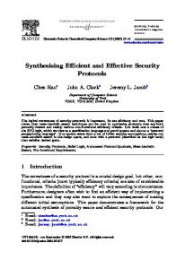
Figure 1. An example of LSH process. tances among objects. It achieves such dimension reduction using a special family of locality sensitive hash functions. The main idea of the LSH is to use the hash functions to map a high-dimensional point to a number of values, such that the points close to each other in their high-dimensional space will have similar values. The points are then classified according to their hashed values. Finally, the near neighbors of a query point can be retrieved by locating points with the similar hashed values. Figure 1 shows an example of the LSH process. It has three components: source records, buckets, and hash tables. Source records are the data records in a database. A bucket is used to denote a group of hash values. A record’s index is its location in the database. LSH stores the indices of similar records in the same group in a final hash table with high probability. Particularly, there are two steps for the data classification in LSH. First, LSH generates L buckets for each record vector. Each bucket corresponds to a final hash table in the L hash tables. That is, the first bucket corresponds to the first hash table, and the second bucket corresponds to the second hash table, and so on. Second, LSH hashes each bucket and saves the index of the record in the group with this hash value in the corresponding hash table in the L hash tables. The details of these two steps are presented in the following. LSH has a family of hash functions consisting of L groups of hash functions, with each group having k hash functions. The hash function is defined as: ha,b (v) = b

a· v + b c, w

where a and b are integer numbers generated by p-Stable distribution [18], and w is a specified real number. For a data record vector represented by v1 , LSH uses the hash function family to get L buckets for v1 . Each bucket has k hash values. For example, in Figure 1, LSH generates L buckets for v1 . Each bucket has k hash values of v1 represented by < h11 , h12 , . . . , h1k >. Thus, one record has hash values represented by hij (1 ≤ i ≤ L, 1 ≤ j ≤ k). Therefore, there are L buckets for each record. In the second step, LSH hashes the values in each

Identifier  vector

LZW

Compressed  Identifier vector

LSH

Figure 2. The process of the combination of LSH and LZW. bucket to a hash value. Thus, a record will have L final hash values. The index of the record will be stored in the corresponding hash table in the L final hash tables. The indices of the records in a hash table are classified into groups based on the final hash values. The indices of records having the same hash value will be in one group. For example, a record’s hash value of its first bucket is 4, then the index of the record will be stored in the group with hash value 4 in the first hash table. As a result, the index of a record will be stored in a group with its bucket i’s hash value in hash table i (1 ≤ i ≤ L). For a query q, LSH generates L hash values for q using the same process. LSH then searches each hash table for the records whose final hash values are the same as q’s. After LSH locates a set of records whose final hash values are the same as q’s, LSH computes the Euclidean Space Distance between the query record and each of the located records. The records with the distances less than a pre-defined distance threshold are regarded as similar records of the query record.

3.2

Optimized Method

LSH-based

Prospecting

One challenge to apply LSH to data prospecting is how to transform a data record to a vector. We derive all unique keywords in the database, and build a keyword list with length m, where m is the total number of the unique keywords in the system. Each data record has an m bit identifier, with each bit corresponding to one keyword. When determining the identifier of a data record, the keyword list is scanned in the top-down manner. If the record has the keyword, it has “1” in the keyword bit. Otherwise, it has “0” in the keyword bit. As a result, a data record has an identifier vector with m bits consisting of “0”s and “1”s. Let’s take an example to explain how LSH generates identifier vectors. Assume that the records in a database are as follows: v1 : Ann Johnson | 16 | Female | 248 Dickson Street v2 : Ann Johnson | 20 | Female | 168 Garland v3 : Mike Smith | 16 | Male | 1301 Hwy v4 : John White | 24 | Male | Fayetteville | 72701 Using the identifier vector generation method intro-

duced, the records have the identifier vectors listed below: v1 : 1 0 0 1 0 0 1 0 0 1 0 1 0 0 1 1 0 0 0 0 v2 : 1 0 0 1 0 0 0 1 0 1 0 0 1 0 0 0 1 0 0 0 v3 : 0 1 0 0 1 0 1 0 0 0 1 0 0 1 0 0 0 1 0 0 v4 : 0 0 1 0 0 1 0 0 1 0 1 0 0 0 0 0 0 0 1 1 A massive database has a large number of unique keywords. Then, each record will have a very long identifier vector. If a record has only a few keywords, it has only a few non-zero bits in its identifier vector. This sparsity leads to inefficiency of Euclidean Space Distance calculation. To optimize the LSH-based prospecting method, we apply the LZW algorithm [17] to LSH to reduce the dimension of the sparse identifier vectors. Figure 2 shows a model of the integration of LZW algorithm to the LSH process. The functionality of LZW is to compress the high-dimensional identifier vectors to low-dimensional identifier vectors. LSH algorithm will then continue to process the low-dimensional identifier vectors. LZW preserves the locality relationship of records, so it will not affect the effectiveness of LSH for data prospecting. Using LZW algorithm, the identifier vectors in the example are changed to: v1 : 12 11 08 07 v2 : 12 11 09 08 v3 : 12 16 18 23 v4 : 13 15 38 27 Thus, LZW compresses the identifier vectors from dimension 20 to dimension 4. After that, LSH hashes each of the compressed v1 , v2 , v3 and v4 into L hash tabes. Assume a query record q is: q: Ann Johnson | 20 | Female | 168 Garland Using the same procedure of generating identifier vectors, q will be transformed to q: 1 0 0 1 0 0 0 1 0 1 0 0 1 0 0 0 1 0 0 0, Then, LZW compressed q to: q: 12 11 09 08. During the query process, LSH generates L hash values for the compressed identifier of q < 12 11 09 08 >. The source records having the same hash values as q’s will be located by LSH as similar records of q. Finally, the Euclidean Space Distance between each located record and the query is computed, and the records with the distance larger than the distance threshold will be removed from the returned record set. Because of the LZW compressing, the dimension of the vector identifiers of the records is much smaller than that before compressing, thus the efficiency of Euclidean Space Distance calculation is improved. For details of the optimized LSH-based prospecting method, please refer to [19].

LSH with LZW

LSH without LZW

70

900 60 Total Query Time (Seconds)

Length of Prospect List

800 700 600 500 400 300 200 100

50 40 30 20 10

0 1

3

5

7

9

11 13 15 17 19 21 23 25 27 29 31 33

0

The Nth Query Record

LSH with LZW

LSH without LZW

Figure 3. Length of prospect list. Figure 4. Total query time.

Performance Evaluation

We conducted experiments on E2LSH 0.1 of MIT [20]. E2LSH 0.1 is a simulator for the highdimensional near neighbor search based on LSH in the Euclidean space. There are 20,591 keywords in the dataset. Therefore, the dimension of the space and the length of every record’s vector is 20,591. There are totally 10,000 source records in the dataset. We randomly selected 97 query records from source records. In the hash function ha,b (v) = b a·v+b w c in LSH, w was set to 4 which is an optimized value [21]. The threshold of Euclidean Space Distance was set to 3 in all experiments. We call each record in a list of located records as prospect, and call a prospect that is a actual neighbor of a query as target prospect. We evaluate the effectiveness of the “LSH with LZW” algorithm in the following metrics in comparison with “LSH without LZW”. • Length of prospect list. Longer prospect list with the same success rate means more false positive results, and less effectiveness of a prospecting method. • Total query time. It shows the efficiency of a prospecting method in terms of prospecting latency. • Memory. It shows the efficiency of a prospecting method in terms of memory requirement. Figure 3 shows the length of the prospect list of a number of randomly selected queries. We can see that the “LSH without LZW” returns much more records than “LSH with LZW”. The results illustrate that by compressing the vectors, LZW can help LSH to remove false positive results. LZW compresses the record vectors while still preserving their relative locations in the mutidimensional space. Thus, “LSH with LZW” improves the accuracy to prospect the nearest neighbors, and discard more results that are not neighbors to the query point. Our experiment results also show that “LSH with LZW” can return most of the target prospects though it

1200000000 1000000000

Memory (Bytes)

4

800000000 600000000 400000000

200000000 0 LSH with LZW

LSH without LZW

Figure 5. Memory consumption. loses a few target prospects. It is in expectation since compression may change the position of a point in the multidimensional space. Considering the reduction of large number of false positive results, “LSH with LZW” should have higher effectiveness rate than “LSH without LZW”. Figure 4 shows the total query time of “LSH with LZW” and “LSH without LZW”. We can find that “LSH with LZW” dramatically reduces the prospecting time of “LSH without LZW”. By compressing record vectors, there will be less hashed values and the sizes of hash tables in LSH are greatly reduced. In addition, the time in the refinement phase is also reduced. Since “LSH with LZW” has fewer operations of hash value comparison and distance calculation, it greatly reduces the total prospecting time of “LSH without LZW”. Figure 5 plots the memory requirements of “LSH with LZW” and “LSH without LZW” in the LSH process. It demonstrates that “LSH with LZW” needs much less memory than “LSH without LZW”. It is due to the reason that “LSH with LZW” has shorter record vectors, and smaller hash tables. Therefore, “LSH with LZW” saves the memory consumption of “LSH without LZW” significantly.

5

Conclusions

This paper presents a method based on Locality Sensitive Hashing (LSH) for data prospecting in a database. Though it has high performance in data prospecting, it incurs low efficiency and effectiveness in large and highdimensional databases. This paper further introduces the use of Lempel-Ziv-Welch (LZW) algorithm to compress dimensionality while still preserving the relative similarities between data records. We integrate LZW into LSH to improve LSH’s efficiency in terms of memory consumption and prospecting latency, and enhance LSH’s effectiveness in successfully locating similar data. Theoretical analysis is presented for the feature of LZW and its effectiveness on LSH. Experiment results show that LSH with LZW algorithm significantly improves the accuracy of located information, and the efficiency of LSH in terms of memory and time requirements.

[7] R. Panigrahy. Nearest neighbor search using kdtrees. Technical report, Stanford University, 2006. [8] S. Arya, D. M. Mount, N. S. Netanyahu, R. Silverman, and A. Wu. An optimal algorithm for approximate nearest neighbor searching. In Proc. 5th ACM-SIAM Sympos. Discrete Algorithms, 1994. [9] A. Fu, P. M. S. Chan, Y. L.Cheung, and Y. S. Moon. Dynamic vp-tree indexing for n-nearest neighbor search given pair-wise distances. VLDB Journal, 9(2):154–173, 2000. [10] P. N. Yianlios. Data structures and algorithms for nearest neighbor search in general metric spaces. In Proc. of the fourth annual ACM-SIAM Symposium on Discrete algorithms, 1993. [11] S. Brin. Near neighbor search in large metric space. In Proc. of the 21st international Conference on VLDB, 1995.

Acknowledgements This research was supported in part by the Acxiom Corporation.

References [1] M. Datar, N. Immorlica, P. Indyk, and V. S. Mirrokni. Locality-sensitive hashing scheme based on p-stable distributions. In Proc. of the 20th annual symposium on Computational geometry (SCG), 2004. [2] J. J. Hu, C. J. Tang, J. Peng, C. Li, C. A. Yuan, and A. L. Chen. A clustering algorithm based absorbing nearest neighbors. In 6th International Conference of WAIM, 2005. [3] D. A. White and R. Jain. Algorithms and strategies for similarity retrieval. Technical Report VCL-96101, University of California, 1996. [4] C. W. Niblack, R. Barber, W. Equitz, M. D. Flickner, E. H. Glasman, D. Petkovic, P. Yanker, C. Faloutsos, and G. Taubin. The QBIC project: querying images by content using color, texture and shape. In Proc. of SPIE: Storage and Retrieval for Image and Video Database, 1993.

[12] Wikipedia. Locality sensitive hashing, 2007. http://en.wikipedia.org/wiki/Locality sensitive hashing. [13] M. Datar, N. Immorlica, P. Indyk, and V. Mirrokni. Locality-sensitive hashing scheme based on p-stable distributions. In Proc. of DIMACS Workshop on Streaming Data Analysis and Mining, 2003. [14] P. Indyk and R. Motwani. Approximate nearest neighbors: Towards removing the curse of dimensionality. In Proc. of the 30th Annual ACM Symposium on Theory of Computing, 1998. [15] V. M. Zolotarev. One-Dimensional Stable Distributions. American Mathematical Society, 1986. [16] H. Shen, T. Li, and T. Schweiger. An Efficient Similarity Searching Scheme Based on Locality Sensitive Hashing. In Proc. of the The Third International Conference on Digital Telecommunications (ICDT), 2008. [17] Terry A. Welch. A Technique for High Performance Data Compression. IEEE Computer, (6):8– 19, 1984.

[5] J. B. Kruskal and M. Wish. Multidimensional scaling. SAGE publication, Beverly Hills, 1978.

[18] A. Fu, P. M. S. Chan, Y. L.Cheung, and Y. S. Moon. Dynamic VP-Tree Indexing for N-Nearest Neighbor Search Given Pair-Wise Distances. VLDB Journal, (2):154–173, 2000.

[6] J. L. Bentle, J. H. Friedman, and R. A. Finkel. An algorithm for finding best matches in logarithmic expected time. ACM Transactions on Mathematical Software, 3(3):209–226, 1977.

[19] H. Shen, T. Li, and Z. Li. Exploring Efficient and Effective LSH-based Methods for Data Prospecting. Technical Report TR-2008-01-90, University of Arkansas, 2008.

[20] A. Andoni. LSH Algorithm and Implementation (E2LSH), 2005. http://web.mit.edu/andoni/www/LSH/index.html. [21] A. Andoni and P. Indyk. E2LSH 0.1 User Manual, 2005. http://web.mit.edu/andoni/www/LSH/index.html.