evaluation of RAxML on the IBM Cell Broadband Engine. .... This Section describes a novel heuristic optimization of the RAxML search algorithm that is available ...
Exploring new Search Algorithms and Hardware for Phylogenetics: RAxML meets the IBM Cell A. Stamatakis1 , F. Blagojevic2 , D.S. Nikolopoulos2 , C.D. Antonopoulos3 1 2
´ School of Computer & Communication Sciences, Ecole Polytechnique F´ed´erale de Lausanne Center for High-end Computing Systems, Department of Computer Science, Virginia Tech 3
Division of Research and Informatics, Greek Armed Forces
Abstract Phylogeny reconstruction is considered to be among the grand challenges in Bioinformatics due to the immense computational requirements. RAxML is currently among the fastest and most accurate programs for phylogenetic tree inference under the Maximum Likelihood (ML) criterion. Initially, we introduce new tree search heuristics that accelerate RAxML by factor 2.43 while returning equally good trees. The performance of the new search algorithm has been assessed on 18 real-world datasets comprising 148 up to 4,843 DNA sequences. We then present the implementation, optimization, and evaluation of RAxML on the IBM Cell Broadband Engine. We address problems and provide solutions pertaining to the optimization of floating point code, control flow, communication, and scheduling of multi-level parallelism on the Cell.
Keywords: Phylogenetic Inference, Maximum Likelihood, RAxML, IBM Cell.
1
Introduction
Phylogenetic trees are used to represent the evolutionary history of a set of n organisms. An alignment with the DNA or protein sequences representing n organisms can be used as input for the computation of phylogenetic trees. In a phylogeny the organisms of the input data are located at the tips (leaves) of the tree whereas the inner nodes represent extinct common ancestors. The branches of the tree represent the time which was required for the mutation of one species into another, new one. Phylogenetic trees have many important applications in medical and biological research (see [2] for a summary). 1
Due to the rapid growth of sequence data over the last years it has become feasible to compute large trees which often comprise more than 1,000 organisms and sequence data from several genes (so-called multi-gene alignments). This means that alignments grow in the number of organisms and in sequence length. The computation of the tree-of-life containing representatives of all living beings on earth is still one of the grand challenges in Bioinformatics. The fundamental algorithmic problem computational phylogeny faces is the immense amount of alternative tree topologies which grows exponentially with the number of organisms n, e.g. for n = 50 organisms there exist 2.84 ∗ 1076 alternative trees (number of atoms in the universe ≈ 1080 ). In fact, it has only recently been shown that the ML phylogeny problem is NP-hard [7]. In addition, ML-based inference of phylogenies is very memoryand floating point-intensive. Since phyloinformatics has definitely entered the HPC era by now, the application of high performance computing techniques as well as the assessment of new CPU architectures can significantly contribute to the reconstruction of larger and more accurate trees. In addition, typical ML implementations exhibit different levels of parallelism and are thus well-suited as example applications for exploiting unconventional and challenging architectures. The Cell Broadband Engine (BE) has been developed jointly by Sony, Toshiba and IBM. Although primarily intended as a processor for Sony PlayStation3, it can theoretically support a broad range of applications. The Cell BE is a heterogeneous multicore processor with nine processing cores: one two-way multithreaded PowerPC Processor Element (PPE) and eight Synergistic Processor Elements (SPEs). The Cell is well suited for data-intensive scientific applications with high demand for memory bandwidth. It offers a unique assembly of MIMD and SIMD execution capabilities and a software-managed memory hierarchy, thus providing ample flexibility in selecting programming and parallelization models for a given application. According to its specifications [1], the Cell is capable of achieving significant performance
2
improvement over conventional multicore CPUs, including an improved power consumption/performance ratio. However, due to its unconventional architecture, the development of parallel applications that can exploit all advantages of the Cell design, is a challenging task. One of the main difficulties is the management of the local storage of the SPEs by software. Another challenge lies in the distribution of work among SPEs, which can be implemented at multiple degrees of granularity and with a variety of code and data distribution schemes, the trends of which are yet to be crystallized. This paper addresses these problems in the realm of algorithms for phylogenetics and more specifically RAxML [27] which is currently among the fastest and most accurate ML algorithms. We present optimizations and system software support for vectorization, control flow parallelization, scheduling, and communication on the Cell, along with a stepwise evaluation of these optimizations in RAxML. The optimizations are generic enough to be reused across a wider range of parallel applications. The remainder of this paper is organized as follows: Initially, we review related work on IBM Cell portings and tools (Section 2). In Section 3 we provide an overview of RAxML and related work in the area of phylogenetics. We also introduce new tree search heuristics that accelerate RAxML by factor 2.43 while returning equally good trees on real-world datasets of 148 up to 4,843 DNA sequences. The following Section 4 gives a step-by-step description of porting and optimizing RAxML on Cell. The conventional optimizations we used to speedup the execution time include the use of optimized numerical libraries for the SPEs, doublebuffering for complete communication/computation overlap, vectorization of floating point operations, and minimization of the ratio of PPE-SPE computation via function off-loading. We also present new Cell-specific optimizations, including the vectorization of conditional statements, asynchronous communication via direct SPE memory accesses and an eventdriven scheduling model, which can selectively exploit coarse-grain and fine-grain parallelism, in response to workload variation. In Section 5 we evaluate performance of RAxML on the IBM Cell and the IBM Power5 multicore processor. We conclude with Section 6.
3
2
Related Work on IBM Cell
Recently, several studies were conducted to measure performance and develop programming models for easier porting as well as optimization of parallel applications on the Cell. Fatahalian et al. [10] developed Sequoia, a programming language suitable for porting memory-aware applications to machines with different memory hierarchy configurations. One of the target architectures in this study is the Cell Broadband Engine. The authors used Sequoia to port several programs to Cell and obtained memory throughput exceeding 20 GB/s. Sequoia currently supports applications which can be parallelized via recursive block decomposition, whereas our work focuses on less structured applications that can be parallelized at multiple layers and where the management of multilevel parallelism can be tedious for the programmer. Bellens et al. [3] developed a dependence-driven programming model for porting sequential applications to Cell. Their compiler is capable of generating tasks that can potentially be executed in parallel. The supporting runtime system creates a dependence graph of active tasks during execution and determines which tasks can be scheduled for execution on the SPEs. This work considers only one layer of task-level parallelism and does not explore the implications of task size and available parallelism within tasks. Both issues are central in the current paper. Kunzman et al. [19] are in the process of adapting Charm++ on Cell. Charm++ is a runtime system for object-based parallel programming. More specifically, Charm++ is a library of machine-independent object abstractions for scheduling and communication on parallel machines, implemented on both distributed and shared memory systems. No results that would enable comparisons with our work are reported as of the time of writing this paper. Although Cell has been a focal point in numerous articles in popular press, published research using Cell for real-world scientific applications beyond games and media-intensive computation is scarce. Besides our study, Hjelte [16] presents an implementation of a smooth 4
particle hydrodynamics simulation on Cell. This simulation requires good interactive performance, since it lies on the critical path of real-time applications such as interactive simulation of human organ tissue, body fluids, and vehicular traffic. Benthin et al. [4] present a parallel ray-tracing algorithm for Cell.
3
The RAxML Application
Despite the high computational cost of ML significant progress has been achieved over the last years in the field of heuristic ML search algorithms with the release of programs such as IQPNNI [21], PHYML [15], GARLI [31] and RAxML [27, 28] to name only a few. RAxML-VI-HPC (v2.2.0) (Randomized Axelerated Maximum Likelihood version VI for High Performance Computing) [27] is a program for large-scale ML-based [13] inference of evolutionary trees using multiple alignments of DNA or AA (Amino Acid) sequences. The program is freely available as open source code at icwww.epfl.ch/˜stamatak. Some of the largest published ML-based biological analyses to date have been conducted with RAxML [11, 14, 23].
The program is also part of the greengenes project [12] (green-
genes.lbl.gov) as well as the CIPRES (CyberInfrastructure for Phylogenetic RESearch, www.phylo.org) project. To the best of our knowledge RAxML-VI-HPC has been used to compute trees on the two largest data matrices analyzed under ML to date: a 25,057-taxon alignment of protobacteria (length: 1,463 nucleotides) and a 2,182-taxon alignment of mammals (length: 51,089 nucleotides). The current version of RAxML (v2.2.0) implements the new search algorithm described in Section 3.2 as well as the older algorithm (command line switch -f o) outlined in [27]. A recent performance study [27] on real world datasets ≥ 1,000 sequences reveals that it is able to find better trees in less time and with lower memory consumption than other current ML programs (IQPNNI, PHYML, GARLI). Moreover, RAxML-VI-HPC has been parallelized with MPI (Message Passing Interface) to exploit the embarrassing parallelism inherent to
5
ML analyses (see Section 3.1). In addition, it has been parallelized with OpenMP [29]. Like every ML-based program, RAxML also exhibits a source of fine-grained loop-level parallelism in the likelihood functions which consume over 90% of the overall computation time. This source of parallelism scales particularly well on large memory-intensive multi-gene alignments due to increased cache efficiency. Finally, RAxML has also recently been ported to a GPU (Graphics Processing Unit) [6].
3.1
The MPI-Version of RAxML
The MPI version of RAxML exploits the embarrassing parallelism that is inherent to every real-world phylogenetic analysis. In order to conduct a “publishable” tree reconstruction (see [14] for an example with RAxML) a certain number (typically 20–200) of distinct tree searches on the original alignment as well as a large number (typically 100–1,000) of bootstrap analyses have to be conducted. Thus, if the dataset is not extremely large this represents the most reasonable approach to exploit HPC platforms. Multiple Inferences on the original alignment are required in order to determine the bestknown ML tree (we use “best-known” because the problem is NP-hard). This is the tree which will be visualized and published. In the case of RAxML each independent tree search starts from a distinct starting tree. This means, that the vast topological search space is traversed from a different starting point every time and will yield final trees with different likelihood scores (see [28] for details on starting tree generation and the search algorithm). Bootstrap Analyses are required to assign confidence values ranging between 0.0 and 1.0 to the inner nodes of the best-known ML tree. This allows to determine how well-supported certain parts of the tree are and is important for the biological conclusions drawn from it. Bootstrapping is essentially very similar to multiple inferences. The only difference is that inferences are conducted on a randomly re-sampled alignment for every bootstrap run, i.e. a certain amount of alignment columns (typically 10–20%) are re–weighted. This is performed in order to assess the topological stability of the tree under slight alterations of the input 6
data. For a typical biological analysis a minimum of 100 bootstrap runs is required. All those individual tree searches, be it bootstrap or multiple inferences are completely independent from each other and can thus be exploited by a simple master-worker scheme.
3.2
Accelerating the Search Algorithm
This Section describes a novel heuristic optimization of the RAxML search algorithm that is available as of version 2.2.0. The entire procedure is outlined in Figure 1. The fundamental mechanism that is used to search the tree space with RAxML is called Lazy Subtree Rearrangement (LSR, for details see [28]). An LSR consists in pruning/removing a subtree from the currently best tree t and then re-inserting it into all neighboring branches up to a certain distance/radius (rearrangement distance) of n nodes from the pruning point (n typically ranges from 5–25). For each possible subtree insertion within the rearrangement distance, RAxML evaluates the log likelihood score of the alternative topology. This is done in a lazy way since only the length of the three branches adjacent to the insertion point/node will be optimized. Thus, an LSR only yields an approximate log likelihood all(t′ ) score for each alternative topology t′ constructed by an LSR from t. However, this all(t′ ) score can be used to sort the alternative topologies. After this fast pre-scoring of a large number of alternative topologies, only a very small fraction of the best-scoring topologies needs to be optimized more exhaustively to improve the overall tree score. One iteration of the RAxML hill-climbing algorithm consists in performing LSRs on all subtrees of a given topology t for a fixed rearrangement distance n. Thereafter, the branches of the 20 best-scoring trees are thoroughly optimized. This procedure of conducting LSRs on all subtrees and then optimizing the 20 best-scoring trees, is performed until no improved tree is encountered. The main idea of the new heuristics is to reduce the number of LSRs performed. This is done by using an empirical cutoff-rule that stops the recursive descent of an LSR into deeper branches at a higher rearrangement distance from the pruning position if they do 7
rearrangement distance Tree t ll(t) pruning point
subtree
prune subtree
Tree t’ LSR: optimize these three branches only
if(d(all(t’), ll(t)) < threshold) skip remainimg rearrangements in current clade
Figure 1: Outline of lazy subtree rearrangements with cutoff procedure
not appear to be promising. Thus, if the approximate log likelihood all(t′ ) for the current rearranged tree t′ is worse than the log likelihood ll(t) of the currently best tree t and if the difference δ(all(t′ ), ll(t)) is larger than a certain threshold lhcutof f the remaining LSRs below that node are omitted. The threshold lhcutof f is determined as follows: During the first iteration of the RAxML search algorithm lhcutof f = ∞ which means that no cutoffs are made. In the course of this first iteration, the differences δi (all(ti ), ll(t)) for all those i = 1...m alternative tree topologies ti where all(ti ) ≤ ll(t) are stored. The threshold lhcutof f Pm
for the next iteration is set to the average of δi , i.e. lhcutof f = (
i=1 δi )/m.
If the search
computes an LSR for which all(t′ ) ≤ ll(t) and δ(all(t′ ), ll(t)) ≥ lhcutof f it will simply skip the remaining LSRs below the current node. Thus, each iteration k of the search algorithm uses a threshold value lhcutof f that has been obtained during the previous iteration k − 1. This allows to dynamically adapt lhcutof f to the specific dataset and to the progress of the search. The omission of a large amount of unnecessary LSRs that have a high probability not to improve the tree yields substantial run time improvements and returns equally good trees at the same time (see Table 1). 8
# Seq 148 218 498 628 994 1512 1780 2000 4114
LH-NEW -69726.05 -134195.92 -219186.90 -50940.81 -348936.85 -273435.30 -178930.53 -364916.18 -325621.05
LH-OLD -69725.55 -134199.30 -219186.90 -50938.29 -348936.85 -273443.51 -178925.02 -364914.44 -325620.54
Speedup 1.83 1.98 2.21 2.68 2.34 2.74 2.95 2.65 2.70
#Seq 150 404 500 714 1288 1604 1908 2554 4843
LH-NEW -39606.06 -156151.42 -85794.87 -148543.21 -395999.61 -167398.16 -149645.43 -318488.01 -748075.04
LH-OLD -39606.06 -156147.25 -85794.87 -148544.48 -395999.61 -167399.43 -149645.43 -318488.01 -748067.23
Speedup 2.00 2.00 2.11 2.51 1.92 3.31 2.89 2.49 2.48
Table 1: Average final log likelihood values and speedups over 10 runs on distinct MP starting trees for 18 real-world datasets 3.2.1
Results
To assess performance of the new heuristics we analyzed 18 real-world datasets comprising 148 to 4,843 sequences from various sources (see Acknowledgment). The computations were performed under the CAT approximation of rate heterogeneity [26], but final tree scores were evaluated with the standard GAMMA model of rate heterogeneity. For each dataset we generated 10 starting trees and executed the old and new RAxML search algorithm on each of those starting trees. We performed a total of 380 ML searches which were executed on the Infiniband cluster at the TU M¨ unchen. The cluster is equipped with 36 quad-CPU 2.4GHz AMD Opteron nodes. Table 1 lists the average final log likelihood values (LH-NEW, LH-OLD) for the old and new versions of the RAxML search algorithm. In addition, it provides the average speedup value per dataset. The average speedup over all datasets is 2.43. The slight variations in likelihood scores are insignificant.
4 4.1
Porting and Optimizing RAxML on Cell The Cell BE
The Cell BE is a heterogeneous multicore processor. The design is inspired by graphics co-processors and similar computation accelerators which are commonly used in game ma9
I/O Controller
PowerPC
SPE
SPE
SPE
SPE
LS
LS
LS
LS
Element Interconnect BUS (EIB)
PPE
Memory Controller
LS
LS
LS
LS
SPE
SPE
SPE
SPE
Figure 2: chines and for media-intensive computations. In contrast to conventional processors, graphics co-processors and accelerators typically provide vast memory bandwidth and vectorization capabilities. Therefore, they are able to execute streaming computation kernels such as encryption/decryption, compression, FIR filters and FFTs far more efficiently,. The Cell BE integrates eight specialized co-processors with a conventional, dual-thread 64-bit processor on the same chip. Cell uses a 64-bit PowerPC core for legacy applications and operating systems. The PowerPC version used on the Cell is a two-way hardware multithreaded processor, capable of thread-level parallelism, process-level parallelism, and software virtualization. The PowerPC core (called Power Processing Element or PPE) is physically surrounded by eight specialized processing cores (called Synergistic Processing Elements, or SPEs). The SPEs are laid out in equal distances around a ring called the Element Interconnect Bus (EIB), which can transmit up to 96 bytes per processor cycle, thus offering a maximum bandwidth of 200 GB/s. The PPE is also connected to the EIB. Cell’s SPEs are based on a simple RISC architecture which can issue up to two instructions per cycle, one of which can be a 128-bit SIMD instruction. Since the SPEs do not include hardware for branch prediction they rely on compiler- or other software-generated schemes to predict the outcome of branches. In its current implementation, the SPE pipeline is optimized for single-precision floating-point vector operations, for which the processor can
10
sustain a maximum throughput of over 230 Gflops. This is an artifact of earlier designs of the processor for game consoles, in which double precision floating-point calculations are far less important than in scientific computing. Nevertheless, double-precision throughput on the Cell still amounts to a respectable 21 Gflops. Upcoming versions of the processor for high-performance computing will resolve this problem1 . Each SPE on the Cell has 128 128-bit general-purpose registers and a software-managed local storage. The use of software-managed local memory is unique in the Cell architecture. In the current version of the processor, each SPE has 256 KB of local storage. This storage is expandable to up to 4 MB. Local storage is locally addressable via direct load and store instructions from the owner SPE and globally accessible from other SPEs and the PPE via DMA requests. Software control of the local storage, instead of a conventional cache organization, enables customized cache placement and replacement policies on the SPEs. The local storage can actually be programmed to operate as a set-associative cache [8]. The SPEs decouple processing from communication, via the use of a memory flow controller (MFC). Each SPE can issue up to 16 concurrent DMA requests, including requests for atomic DMA operations, which can be used in lieu of conventional synchronization mechanisms such as locks and requests for scatter-gather memory operations.
4.2
RAxML Porting Strategy
We followed a three-step process for porting RAxML to Cell: 1. We identified and off-loaded the compute intensive parts of RAxML to the SPEs. 2. We optimized the off-loaded code on the SPEs. We used optimized numerical libraries for the SPEs, double buffering, vectorization of computation, vectorization of control flow, and communication optimizations for latency overlap. 1
Personal communication with Kevin Barker, Roadrunner Performance Evaluation Team Member, Los Alamos National Lab.
11
3. Finally, we developed an event-driven scheduler for RAxML’s nested parallel code, along with the necessary system software support. The first two steps follow the function off-loading programming model, which arguably provides the easiest path for porting MPI applications on the Cell [8, 9]. The last step is a new contribution to support the execution of parallel programs with multiple levels of parallelism on the Cell. In the following Sections we describe the porting and optimization process, together with speedups obtained at each optimization step.
4.3
Porting the MPI Code
The version of RAxML that we ported on Cell is based on the new, improved search heuristics, described in Section 3.2. We initially executed the MPI version of RAxML on the PPE. Since the PPE is a dual-threaded processor, the PPE can execute two MPI processes simultaneously. These processes share the resources of the PPE, except from the register file. Therefore, their parallel execution on the PPE is not expected to scale as well as on a 2-way SMP. Although it is natural to consider using the PPE for direct porting of MPI code without modifications, this approach is clearly suboptimal. Due to the heterogeneity of the Cell, further steps are needed to off-load and optimize most, if not all, of the computation within each MPI process, in order to exploit the computational capacity of the SPEs. We explored two strategies for off-loading code on the Cell SPEs. The first strategy is pure task-level off-loading. Each MPI process running on the PPE off-loads functions on the SPEs and each function executes from start to finish on the SPE it is assigned to. The second strategy is a hybrid task-level and loop-level parallelization scheme. Functions are off-loaded from the MPI process to some of the SPEs. The remaining SPEs are used for work sharing of parallel loops included in the already off-loaded functions. These parallelization strategies are described further in Section 4.7.
12
4.4
Selecting Functions for Off-Loading
In order to find the functions in RAxML that are suitable for SPE execution, we profiled the code using gprof. For all the profiling and benchmarking runs of RAxML presented in this paper, we use the input file 42 SC, which contains 42 organisms, each represented by a DNA sequence of 1167 nucleotides. The number of distinct data patterns in a DNA alignment is in the order of 250. Profiling the sequential version of RAxML on the IBM Power5 processor shows that 96.6% of the execution time is spent in four functions: • 64.62% of the time is spent in the function newview(). This function computes the partial likelihood vector [13] at an inner node of the phylogenetic tree. • 26.88% of the time is spent in makenewz(). This function optimizes the length of a given branch with respect to the tree likelihood using the Newton–Raphson method. • 2.87% of the time is spent in newviewPartial(), which optimizes the per-site evolutionary rates for the GTRCAT approximation (see [26] for details) • Finally, 2.29% of the time is spent in evaluate(). This function calculates the Log Likelihood score of the tree at a given branch by summing over the partial likelihood vector entries. Note that the log likelihood value is the same at all branches of the tree if the model of nucleotide substitution is time-reversible [13]. The prerequisite for computing evaluate() and makenewz() is that the likelihood vectors at the nodes to the right and left of the branch have been computed. Thus, makenewz() and evaluate() initially make calls to newview() before they can execute their own computation.
The newview() function at an inner node p calls itself recursively when the two children r and q are not tips (leaves) and the likelihood array for r and q has not already been computed.
Consequently, the first candidate for off-loading is newview(). Although makenewz() and evaluate() are both taking a smaller portion of execution time than newview(), offloading
these two functions can also lead to significant speedup (see Section 4.6). Besides the fact 13
that each function can be optimized and executed faster on an SPE, having all four functions offloaded to an SPE significantly reduces the amount of PPE-SPE communication. The code executed on the SPE has to be compiled separately (using the SPE specific compiler) from the code executed on the PPE. We choose to include all four off-loaded functions in one code module. This approach has the advantage of having all off-loaded functions in the SPE’s local storage during the entire execution of the program. Consequently, an offloaded function can be invoked without introducing the overhead of moving its code from global memory to local storage. However, this decision imposes a trade-off, since the extended code segment in the SPE local storage reduces the available space for the heap and stack segments. In the case of RAxML, the total size of all four off-loaded functions is 110 KB. The remaining space (146 KB) is large enough to store the heap and stack segments of each of the four functions, as well as the buffers needed for communication-computation overlap. To keep the implementation simple, the call to each off-loaded function in the original MPI code is executed with the same signature on the PPE in the Cell code. We replaced the original body of each function with communication code needed to transfer local data used in the function from the PPE to SPEs. Whenever an off-loaded function is called, the PPE sends a signal to the SPE thread and waits for the SPE thread to complete the function and return the result. While waiting for the SPE code to finish, the PPE seeks functions for off-loading from other MPI processes. This process is described in more detail in Section 4.7. All four off-loaded functions are executed inside a single SPE thread. The SPE thread is created at the beginning of the program and stays alive during the entire program execution. Depending on the content of a triggering signal received from the PPE, the thread executes one of the four offloaded functions. By having a single thread active during the entire program execution, we avoid excessive overhead from repeated spawning and joining of threads. The SPE threads execute a busy wait for a PPE signal.
14
Data consistency is maintained at the granularity of off-loaded functions. Each function is individually responsible for collecting local updates and propagating these updates to global shared memory.
4.5
Optimizing Off-Loaded Functions by Example of
newview()
Since newview() is the most computationally expensive function in the code, it becomes the first candidate for optimization. We found that na¨ıvely off-loading newview() slows down the sequential version of the code by a factor of 2.8. Therefore, exhaustive optimization of the function on the SPE was necessary. Table 2 summarizes the execution times of RAxML before and after newview() is off-loaded. The first column shows the number of workers (MPI processes) used in the experiment and the amount of work done (number of bootstraps).
(a)
1 2 2 2
worker, 1 bootstrap workers, 8 bootstraps workers, 16 bootstraps workers, 32 bootstraps
28.3s 152.56s 309.53s 622.43s
(b)
1 2 2 2
worker, 1 bootstrap workers, 8 bootstraps workers, 16 bootstraps workers, 32 bootstraps
80.52s 348.36s 696.12s 1375.09s
Table 2: Execution time of RAxML (in seconds). The input file is 42 SC: (a) The application is executed on the PPE, (b) newview(), without optimizations, is offloaded to one SPE. We profiled the function newview() using the special decrementer register of the SPE. We identified four code segments that consume almost the entire execution time in newview(): 1. Math library functions, such as exp() and log(). These functions are very expensive if their native implementations are executed on the SPE. In newview(), the exp() function is used to compute the transition probabilities of the nucleotide substitution matrix for the branches from the root of a subtree to its descendants. The log() function is used to scale the branch lengths for numerical reasons [25]. 2. An if(. . .) statement in the code which determines the value of a conjunction of four expressions is the second bottleneck. This conditional statement is used to check if
15
small likelihood vector entries need to be scaled to avoid numerical underflow (similar operations are used in every ML implementation). 3. Blocking DMA requests also have a significant impact on execution time. Whenever data required for the computation is not in local storage, the program has to wait for the necessary data to be fetched from global memory. 4. All double precision floating point arithmetic used for the likelihood vector calculation is not natively vectorized or optimized. In the next few subsections we describe performance optimizations for the off-loaded newview() function. We applied analogous optimizations to the remaining off-loaded func-
tions. We do not discuss the other functions in more detail due to space limitations. 4.5.1
Mathematical Functions
The first step in reducing the execution time of the off-loaded function was to replace the expensive math functions exp() and log() with the mathematical functions provided by the Cell SDK 1.1. The exp() and log() functions provided by the Cell SDK are implementations of numerical methods for exponent and logarithm calculation. The exp() and log() functions represent less than 1% of the total number of floating point operations executed in the off-loaded function, however they account for 56% of execution time in newview(). Using the implementations of the exponent and logarithm functions provided by the Cell SDK improves total execution time by 37% - 41%. Table 3 shows the execution times of the four test runs of RAxML after newview() is off-loaded and exp() and log() functions are replaced with optimized implementations. Notice that the off-loaded code is still 40%–47% slower than the non off-loaded code.
16
(b)
1 2 2 2
worker, 1 bootstrap workers, 8 bootstraps workers, 16 bootstraps workers, 32 bootstraps
47.94s 218.17s 433.94s 871.49s
Table 3: Execution time of RAxML with no off-loading (a), and with newview() off-loaded and optimized to use numerical functions from the SDK library. The input file is 42 SC. 4.5.2
Optimizing Conditional Statements
Function newview() is always invoked at an inner node of the tree (p) which is at the root of a subtree. The main computational kernel of newview() has a switch statement which selects one out of four paths of execution. If one or both descendants r and q of p are tips (leaves) the computations of the main for-loop in newview() can be simplified. This optimization leads to significant performance improvements [27]. Thus, there are distinct implementations of the main computational part of newview() for the case that r and q are tips, r is a tip, q is a tip, or r and q are both inner nodes. Each path in the switch statement leads to a large loop which performs the likelihood vector calculations. Each iteration of the large loop executes a large if() statement which determines the value of a conjunction of four arithmetic expressions. This conditional statement checks if likelihood scaling is required to prevent numerical underflow. On an SPE, a mispredicted branch incurs a penalty of 20 cycles [17]. Using the decrementer register to profile the off-loaded code, and after optimization of exp() and log()), we find that 39% of the execution time of newview() is spent in checking the condition of the if() statement executed in the likelihood vector calculation loop. The conditional statement is shown in Figure 3. minlikelihood is a positive constant and all operands are double precision floating point values. The ABS() function increases the number of condition checking (each ABS() function executes an additional comparison), therefore the number of conditions that need to be checked in this statement is actually eight.
17
if (ABS(x3->a) < minlikelihood && ABS(x3->g) < minlikelihood && ABS(x3->c) < minlikelihood && ABS(x3->t) < minlikelihood) { . . . }
Figure 3: Conditional statement which takes 39% of newview() execution time, after optimization of numerical functions. On an SPE, two integer numbers can be compared significantly faster than two double precision floating point numbers. The advantage of integers is that they can be compared using the existing SPE intrinsics. Current SPE intrinsics support comparison of at most 32bit integer values. 64-bit large integers can also be compared relatively fast, by combining 32bit integer intrinsics. The spu-gcc compiler automatically optimizes conditional statements that operate on integer values, by replacing them with suitable SPE intrinsics. According to the IEEE standard, all double precision floating point numbers are “lexicographically ordered”. In other words, if two double floating point numbers a and b are ordered (a < b), then their bit patterns will be ordered in the same way when interpreted as Sign-Magnitude integers [18] (*(unsigned long long*)&a < *(unsigned long long*)&b). However, this rule can only be applied if both numbers are larger than 0. In the conditional statement that we are trying to optimize all parameters are greater than 0 (we know that minlikelihood is a constant greater than 0). Therefore, instead of comparing double precision floating point values, we can optimize the problematic if() statement by casting all our operands to unsigned long long before comparing them. To avoid the branch used in the ABS() function,
we transform all our operands to positive numbers, using a bitwise AND. This optimization reduces the time spent in the conditional statement to only 7% of the execution time of newview(). The total execution time of RAxML is reduced by 20%. Table 4 shows the new execution times of RAxML after optimizing both conditional statements and numerical functions in newview().
18
1 2 2 2
(b)
worker, 1 bootstrap workers, 8 bootstraps workers, 16 bootstraps workers, 32 bootstraps
38s 177.68s 354.85s 703.95s
Table 4: Execution time of RAxML after the floating-point conditional statement is transformed to an integer conditional statement. The input file is 42 SC. 4.5.3
Double Buffering and Memory Management
The number of iterations in the main loop of newview() depends on the input alignment length. This loop operates on three arrays with equal length (likelihood vector at current subtree root, and likelihood vectors at left and right child). The loop has no loop-carried dependencies and executes as many iterations as the length of the three arrays. Since the size of the local storage is only 256 KB, the arrays cannot be stored permanently in local storage. Instead, the arrays are strip-mined and processed in blocks. The block size is selected such that the computation on a block can overlap completely with the memory latency for fetching the next block. We use a 2 KB buffer for caching each array block, which holds enough data to execute 16 loop iterations. We also use double buffering to mask memory latency, which amounts to 8% of the execution time of the code before optimization. Table 5 shows the improved execution times of RAxML after optimization of numerical operations, optimization of conditionals and memory latency overlap, which improved total execution time by 3–5%. 1 2 2 2
worker, 1 bootstrap workers, 8 bootstraps workers, 16 bootstraps workers, 32 bootstraps
36.29s 169.50s 338.24s 688.04s
Table 5: Execution time of RAxML with double buffering applied to overlap DMA transfers with computation, after optimization of numerical functions and conditionals. The input file is 42 SC.
19
4.5.4
Vectorization
The core of the computation in newview() is concentrated in two loops. The first loop is executed at the beginning of the function and computes the individual transition probability matrices for each distinct rate category of the CAT model [26]. The number of iterations is relatively small (between 1 and 25) and each iteration executes 36 double precision floating point operations. The second loop calculates the likelihood vector. The length of this vector corresponds to the number of distinct alignment patterns. Each iteration of this loop executes 44 double precision floating point operations for the CAT model. The kernel of the first loop in newview() is shown in Figure 4(a). In Figure 4(b) we (a)
(b)
for( ... ) { ki = *rptr++;
1: vector double *left_v = (vector double*)left; 2: vector double lz1011 = (vector double)(lz10,lz11); . . .
d1c = exp (ki * lz10); d1g = exp (ki * lz11); d1t = exp (ki * lz12); *left++ = d1c * *EV++; *left++ = d1g * *EV++; *left++ = d1t * *EV++; *left++ *left++ *left++ .
= = = .
for( ... ) { 3: ki_v = spu_splats(*rptr++); 4:
d1c * *EV++; d1g * *EV++; d1t * *EV++; .
d1cg = _exp_v ( spu_mul(ki_v,lz1011) ); d1tc = _exp_v ( spu_mul(ki_v,lz1210) ); d1gt = _exp_v ( spu_mul(ki_v,lz1112) ); left_v[0] left_v[1] left_v[2] .
}
= = = .
spu_mul(d1cg,EV_v[0]); spu_mul(d1tc,EV_v[1]); spu_mul(d1gt,EV_v[2]); .
}
Figure 4: The body of the first loop in newview(): (a) Non–vectorized code, (b) Vectorized code. show the same code vectorized for the SPE. The function spu mul() multiplies two vectors (in this case the arguments are vectors of doubles). Function exp v() is the vector version of the exponential function mentioned in Section 4.5.1. After vectorization, the number of floating point operations executed in the body of the first loop drops from 36 to 24. An additional instruction is required to create a vector from a scalar element. Due to pointer arithmetic on dynamically allocated data structures, automatic vectorization of this code 20
would be particularly challenging for a compiler. The second loop is vectorized in a similar way. Figure 5 shows the core of the second loop before and after vectorization. The variables x1->a, x1->c, x1->g, x1->t, belong to (a)
(b)
for( ... ) { ump_x1_0 ump_x1_0 ump_x1_0 ump_x1_0
for( ... ) { a_v = spu_splats(x1->a); c_v = spu_splats(x1->c); g_v = spu_splats(x1->g); t_v = spu_splats(x1->t);
ump_x1_1 ump_x1_1 ump_x1_1 ump_x1_1
= x1->a; += x1->c * *left++; += x1->g * *left++; += x1->t * *left++;
= += += += . .
x1->a; x1->c * *left++; x1->g * *left++; x1->t * *left++; .
l1 = (vector double)(left[0],left[3]); l2 = (vector double)(left[1],left[4]); l3 = (vector double)(left[2],left[5]); ump_v1[0] ump_v1[0] ump_v1[0] .
}
= = = .
spu_madd(c_v,l1,a_v); spu_madd(g_v,l2,ump_v1[0]); spu_madd(t_v,l3,ump_v1[0]); .
}
Figure 5: Core of likelihood calculation loop in newview(): (a) Non–vectorized code, (b) Vectorized code. the same C structure (likelihood vector) and are stored in contiguous memory locations. In Figure 5 (a) we see that only three of these variables are multiplied with the elements of array left. Therefore, vectorization cannot be accomplished by simply interpreting the members of the likelihood vector structure that reside in consecutive memory locations as vectors. We actually need to create vectors using special intrinsics for vector creation, such as spu splats(). Vectorization decreases the execution time of the two major loops in newview() from 12.8 seconds to 7.3 seconds. Table 6 summarizes the execution times for RAxML, after vectorization, optimization of numerical functions, optimization of conditional statements and optimization for memory latency overlap in newview(). After vectorization, the code which off-loads newview() on the SPE becomes up to 7% faster than the code without offloading.
21
1 2 2 2
worker, 1 bootstrap workers, 8 bootstraps workers, 16 bootstraps workers, 32 bootstraps
30.13s 143.20s 287.31s 577.1s
Table 6: Execution time of RAxML after vectorization, optimization of numerical functions, optimization of conditionals and optimization for memory overlap. The input file is 42 SC. 4.5.5
PPE-SPE Communication
Although newview() dominates the execution time of RAxML, each instance of the function executes for only 82ms on average. This means that the granularity of the function is small and function invocation overhead when the function is off-loaded on the SPE is by no means negligible, since it requires PPE to SPE communication. For our test dataset, the function is called 178,244 times. We originally implemented PPE to SPE communication using mailboxes, which offer a programmable, high-level interface for communication via message queues. After further experimentation, we found that that DMA transfers achieved lower latency than using mailboxes and improved application execution time by a further 2%-11% in our test cases. Table 7 shows the execution times of RAxML when DMA transfers are used instead of mailboxes and after all optimizations described so far. The input dataset is 42 SC. 1 2 2 2
worker, 1 bootstrap workers, 8 bootstraps workers, 16 bootstraps workers, 32 bootstraps
29.9s 126.87s 253.67s 514.89s
Table 7: Execution time of RAxML after optimizing communication to use DMA transfers and all previously described optimizations. The input file is 42 SC. It is interesting to note that direct memory-to-memory communication is an optimization which scales with parallelism on Cell, i.e. the impact on performance improves as the code uses more SPEs. As the number of workers and bootstraps executed on the SPEs increases, the code becomes more communication-intensive, due to the fine granularity of the offloaded 22
functions. Fast communication by DMA therefore becomes critical.
4.6
Off-Loading Remaining Functions
After off-loading and optimizing the newview() function, we proceeded with off-loading the three remaining compute-intensive functions: makenewz(), evaluate(), and newviewPartial(). Off-loading makenewz() and evaluate() was straightforward. We repeated the same offloading procedure and analogous optimizations as with newview(). As described in Section 4.4, all off-loaded functions are written to the same SPE code module. In this way the off-loaded code remains in the local storage during the entire execution of the application. Consequently, we avoid the cost of repeatedly loading different code modules into local storage. Moreover, we reduce PPE-SPE communication, since each invocation of newview() by either makenewz() or evaluate(), can be performed locally on an SPE without involving the PPE. Off-loading newviewPartial() was a more challenging task. This function is used to recompute the per-site log likelihood values lli at column i of the alignment given a rate ri during the per-site evolutionary rate optimization process (see [26] for details). Since optimizing the ri implies changes of the likelihood vector values at position i in the entire tree, a complete tree traversal (as opposed to a partial tree traversal induced by LSRs as described in Section 3.2) must be carried out to obtain the lli for ri at each alignment position i. Some changes in the data structures were required to allow for future parallel execution of newviewPartial(). Instead of using the likelihood vector arrays allocated for computations over the whole alignment length with newview(), makenewz(), and evaluate() each recursive invocation of newviewPartial() uses the heap to create a private local likelihood vector of length one. These changes enable the concurrent computation of individual per-site log likelihood values lli , llj at distinct alignment positions i 6= j with different rates ri , rj . Due to the fine granularity of newviewPartial() which only operates on one single alignment position and the high amount of calls per alignment position (the ri are optimized in a 23
Brent-like procedure [26]) we off-loaded the large for-loop that optimizes all ri in optimizeRateCategories() to the SPE. This large for-loop has already been parallelized in the current
OpenMP version of RAxML using the OpenMP schedule(dynamic) clause. Dynamic scheduling avoids potential load imbalance because the optimization of each ri requires a different number of iterations until convergence. The parallelization of newviewPartial() with OpenMP yielded a performance improvement of 16% on the 404 sequence dataset with 7,429 distinct patterns from Table 1 on a 4-way AMD Opteron. This large performance improvement is due to the fact that newviewPartial() consumes a significantly larger part of execution time for long multi-gene alignments. With all four functions off-loaded and optimized on the SPE, the application was performing 34%-36% faster. Compared to the initial code which is entirely executed on the PPE, the optimized code is 29% faster. When more than one MPI processes is used and more than one bootstrap is offloaded to SPEs, the gains from offloading reach 47%. Table 8 summarizes the execution times for RAxML when all four functions are off-loaded and optimized for the 42 SC dataset. 1 2 2 2
worker, 1 bootstrap workers, 8 bootstraps workers, 16 bootstraps workers, 32 bootstraps
20.4s 84.41s 165.3s 330.62s
Table 8: Execution time of RAxML after offloading and optimizing four functions: newview(), makenewz(), evaluate() and evaluatePartial(). The input file is 42 SC.
4.7
Scheduling Multilevel Parallelism
The distribution of resources on the Cell often introduces an imbalance between computation supply and demand. The processor has eight SPEs, however, at most two threads can off-load code from the PPE to the SPEs at the same time. To overcome this limitation, we explored an event-driven programming model and the associated system software support. In this
24
model, we allow an arbitrary number of MPI processes to share the PPE and implement a context switching strategy which opts for switching the context of a PPE thread upon off-loading a function from the current context, in anticipation of more opportunities for function off-loading in other contexts. The intuition is that off-loading a function from a PPE thread is typically followed by idle time on the PPE thread, which can be overlapped with computation originating in other PPE threads. We have extended our event-driven scheduling model with an algorithm which tracks SPE utilization and assigns SPEs to off-loaded functions based on utilization. More specifically, each function receives one or more SPEs, which can be used for parallelization of loops enclosed in the function, with mechanisms and policies similar to those of OpenMP. The assignment of SPEs to functions depends on the number of SPEs which are idling during a predefined interval of recent execution. More details on our event-driven model are provided in [5]. The new scheduling model reduces the execution time of one bootstrap by 36%, compared to our original static off-loading scheme, with all SPE-specific optimizations integrated in the code. The reason for the high speedup is the ability to distribute loops inside offloaded functions across SPEs. When loop parallelism and task parallelism are exploited simultaneously in off-loaded functions, the execution time is reduced by up to 63%. Table 9 summarizes the execution times of the optimized implementation of RAxML with our eventdriven programming and scheduling model. 1 bootstrap 8 bootstraps 16 bootstraps 32 bootstraps
14.1s 26.7s 53.63s 107.2s
Table 9: Execution time of RAxML with the event-driven programming and scheduling model (MGPS) is used. The input file is 42 SC. The number of workers is variable and is selected at runtime by the scheduler.
25
5
Comparison with the IBM Power5
It is useful to compare the performance of the Cell against other multicore processors, since such a comparison provides valuable insight both for application developers working on adapting their software to emerging computer architectures, and to computer architects who are looking into improving their hardware to address the needs of challenging applications. In this Section we compare the performance of Cell against an IBM Power5, using our test runs of RAxML. The IBM Power5 is a homogeneous dual-core processor, where each core is itself a two-way simultaneous multithreaded processor. Porting the MPI version of RAxML to the Power5 is straightforward, since all that needs to be done is load four MPI processes (workers) on the four execution contexts of the processor. The Power5 used for this experiment runs at 1.65 GHz, and has 32KB of L1-D and L1-I cache, 1.92 MB of L2 cache and 36 MB of L3 cache. Figure 6 provides the execution times on the two processor types for up to 128 bootstraps, a scale which is more representative of real-world data sets for RAxML. The Cell outperforms the IBM Power5 by 15% on average. Although the difference seems small, a number of considerations should be taken into account. The Power5 has a lower clock frequency, but significantly more secondary and tertiary cache space available to each core. Furthermore, double-precision floating point arithmetic is unoptimized on the Cell’s SPE pipelines, leading to a markedly large reduction in processor throughput (up to a factor of 10) compared to single-precision floating point arithmetic. Furthermore, hardware studies of the Cell indicate that the processor is significantly more power-efficient than the Power5, claiming nominal power consumption in the range of 27W to 43W for the 3.2 GHz model used in this study [30], as opposed to a reported 150W for the Power5 [20]. Taking these observations into consideration, we conclude that the Cell provides a leap forward in performance compared to homogeneous, general-purpose multicore processors. Our study is the first to demonstrate this leap using complex, non-trivial parallel code from the field of computational biology.
26
500 RAxML on IBM RAxML on Cell
Execution time in seconds
450 400 350 300 250 200 150 100 50 0 0
20
40
60
80
100
120
140
Number of bootsrtaps
Figure 6: RAxML performance on a multi-core IBM Power5 and the IBM Cell. The number of bootstraps performed covers 1, 8, 16, 32, 64 and 128 runs.
6
Conclusion and Future Work
We presented an improved heuristic search algorithm for RAxML as well as a detailed stepby-step description of porting RAxML to IBM Cell. The incremental parallelization and optimization methodology presented in this paper can serve as a guideline for parallelization of non-trivial applications on Cell. The optimizations and system software for multilevel parallelization introduced in this paper resolve bottlenecks which are common to many applications and even multicore architectures other than the Cell. The porting strategy and methods developed for exploiting fine-grain parallelism in RAxML on the Cell are generally applicable to a broad range of programs for ML-based (GARLI [31], IQPNNI [21], PHYML [15]) and Bayesian (MrBayes [24]) phylogenetic inference. All these programs spend 90-95% of their total execution time for the evaluation of the likelihood function and face similar problems with respect to memory transfer and function optimization. The strategies and scheduling techniques for coarse-grain parallelism are—with some modifications—also applicable to the MPI-versions of GARLI and IQPNNI. In fact, there already exist a hybrid MPI/OpenMP version of IQPNNI [22] and an OpenMP parallelization of PHYML (Michael Ott, personal communication). Future work will focus on improved ways to handle recursions on SPEs which will allow for inference of large real-world datasets.
27
Acknowledgments We would like to thank Olaf Bininda-Emonds, Nicolas Salamin, Josh Wilcox, Daniel Dalevi, Usman Roshan, Chuck Robertson, and Markus G¨oker for letting us use their often tediously hand-aligned sequence data to assess RAxML performance.
References [1] Cell
broadband
engine
programming
tutorial
version
1.0;
http://www-106.
ibm.com/developerworks/eserver/library/es-archguide-v2.html. [2] D.A. Bader, B.M.E. Moret, and L. Vawter. Industrial applications of high-performance computing for phylogeny reconstruction. In Proc. of SPIE ITCom, volume 4528, pages 159–168, 2001. [3] P. Bellens, J.M. Perez, R.M. Badia, and J. Labarta. Cellss: A programming model for the cell be architecture. In Proceedings if IEEE/ACM Supercomputing conference (SC2006), 11 2006. [4] C. Benthin, I. Wald, M. Scherbaum, and H. Friedrich. Ray Tracing on the CELL Processor. Technical Report, inTrace Realtime Ray Tracing GmbH, No inTrace-2006001 (submitted for publication), 2006. [5] F. Blagojevic, D.S. Nikolopoulos, A. Stamatakis, and C.D. Antonopoulos. Dynamic Multigrain Parallelization on the Cell Broadband Engine. In Proceedings of the 2007 ACM SIGPLAN Symposium on Principles and Practice of Parallel Programming, San Jose, CA, March 2007. [6] M. Charalambous, P. Trancoso, and A. Stamatakis. Initial experiences porting a bioinformatics application to a graphics processor. In Proceedings of the 10th Panhellenic Conference on Informatics (PCI 2005), pages 415–425, 2005. 28
[7] B. Chor and T. Tuller. Maximum likelihood of evolutionary trees: hardness and approximation. Bioinformatics, 21(1):97–106, 2005. [8] A.E. Eichenberger et al. Optimizing Compiler for a Cell processor. Parallel Architectures and Compilation Techniques, September 2005. [9] D. Pham et al. The Design and Implementation of a First Generation Cell Processor. Proc. Int’l Solid-State Circuits Conf. Tech. Digest, IEEE Press, pages 184–185, 2005. [10] K. Fatahalian et al. Sequoia: Programming the memory hierarchy. In Proceedings if IEEE/ACM Supercomputing conference (SC2006), 11 2006. [11] R. E. Ley et al. Unexpected diversity and complexity of the guerrero negro hypersaline microbial mat. Appl. Envir. Microbiol., 72(5):3685 – 3695, May 2006. [12] T.Z. DeSantis et al. Greengenes, a Chimera-Checked 16S rRNA Gene Database and Workbench Compatible with ARB. Appl. Environ. Microbiol., 72(7):5069–5072, 2006. [13] J. Felsenstein. Evolutionary trees from DNA sequences: a maximum likelihood approach. J. Mol. Evol., 17:368–376, 1981. [14] G. W. Grimm, S. S. Renner, A. Stamatakis, and V. Hemleben. A nuclear ribosomal dna phylogeny of acer inferred with maximum likelihood, splits graphs, and motif analyses of 606 sequences. Evolutionary Bioinformatics Online, 2:279–294, 2006. [15] S. Guindon and O. Gascuel. A simple, fast, and accurate algorithm to estimate large phylogenies by maximum likelihood. Syst. Biol., 52(5):696–704, 2003. [16] N. Hjelte. Smoothed Particle Hydrodynamics on the Cell Brodband Engine. Masters Thesis, June 2006. [17] IBM. Cbe tutorial v1.1. 2006.
29
[18] W. Kahan. Lecture notes on the status of ieee standard 754 for binary floating-point arithmetic. 1997. [19] D. Kunzman, G. Zheng, E. Bohm, and L.V. Kal´e. Charm++, Offload API, and the Cell Processor. In Proceedings of the Workshop on Programming Models for Ubiquitous Parallelism, Seattle, WA, USA, September 2006. [20] Sun Microsystems. cember 2005.
Sun UltraSPARC T1 Cool Threads Technology.
De-
http://www.sun.com/aboutsun/media/presskits/ networkcomput-
ing05q4/T1Infographic.pdf. [21] B.Q. Minh, L.S. Vinh, A.v. Haeseler, and H.A. Schmidt. pIQPNNI: parallel reconstruction of large maximum likelihood phylogenies. Bioinformatics, 21(19):3794–3796, 2005. [22] B.Q. Minh, L.S. Vinh, H.A. Schmidt, and A.v. Haeseler. Large maximum likelihood trees. In Proceedings of the NIC Symposium 2006, pages 357–365. Forschunungszentrum J¨ ulich, 2006. [23] C.E. Robertson, J.K. Harris, J.R.Spear, and N.R. Pace. Phylogenetic diversity and ecology of environmental Archaea. Current Opinion in Microbiology, 8:638–642, 2005. [24] F. Ronquist and J.P. Huelsenbeck. MrBayes 3: Bayesian phylogenetic inference under mixed models. Bioinformatics, 19(12):1572–1574, 2003. [25] A. Stamatakis. Distributed and Parallel Algorithms and Systems for Inference of Huge Phylogenetic Trees based on the Maximum Likelihood Method. PhD thesis, Technische Universit¨at M¨ unchen, Germany, October 2004. [26] A. Stamatakis. Phylogenetic models of rate heterogeneity: A high performance computing perspective. In Proceedings of 20th IEEE/ACM International Parallel and Dis-
30
tributed Processing Symposium (IPDPS2006), High Performance Computational Biology Workshop, Proceedings on CD, Rhodos, Greece, April 2006. [27] A. Stamatakis. RAxML-VI-HPC: maximum likelihood-based phylogenetic analyses with thousands of taxa and mixed models. Bioinformatics, 22(21):2688–2690, 2006. [28] A. Stamatakis, T. Ludwig, and H. Meier. RAxML-III: A Fast Program for Maximum Likelihood-based Inference of Large Phylogenetic Trees. Bioinformatics, 21(4):456–463, 2005. [29] A. Stamatakis, M. Ott, and T. Ludwig. RAxML-OMP: An Efficient Program for Phylogenetic Inference on SMPs. PaCT, pages 288–302, 2005. [30] D. Wang. Cell Microprocessor III. Real World Technologies, July 2005. [31] D. Zwickl. Genetic Algorithm Approaches for the Phylogenetic Analysis of Large Biologiical Sequence Datasets under the Maximum Likelihood Criterion. PhD thesis, University of Texas at Austin, April 2006.
31