Exploring relationships between ENSO and ... - Semantic Scholar

int. j. remote sensing, 2001, vol. 22, no. 16, 3077 –3092

Exploring relationships between ENSO and vegetation vigour in the south-east USA using AVHRR data J. MENNIS Department of Geography, The Pennsylvania State University, 302 Walker Building, University Park, PA 16802, USA; e-mail: [email protected] (Received 1 March 1999; in nal form 3 February 2000) Abstract. This research explores the relationship between El Ninõ/Southern Oscillation (ENSO), captured by equatorial Paci c Ocean Sea Surface Temperature (SST), and interannual variation in vegetation vigour in the southeast USA, captured by Advanced Very High Resolution Radiometer (AVHRR) Normalized DiVerence Vegetation Index (NDVI), for the period 1982–1992. The moving average and ‘baseline’ methods (anomaly from the long term mean) were used to extract interannual patterns in the NDVI signature for croplands, deciduous forests and evergreen forests. The ENSO cycle was measured using mean SST anomalies and the percentage of SST cells above certain threshold values (e.g. 1.0° C above the long term mean). The baseline method indicated a weak, yet persistent, negative correlation between ENSO warm phase events and vegetation vigour in the south-east USA. The moving average method yielded similar results but produced higher correlation values ( 0.45 to 0.76, signi cant at the 0.01 level ). Use of the 2.0° C threshold SST anomaly was found to yield the highest correlation values as it captures not only the presence but also the intensity of ENSO warm phase events. These results indicate that there is a clear and recognizable, though inconsistent, relationship between ENSO and vegetation vigour in the south-east USA.

1.

Introduction Understanding the complex relationships between climate and vegetation dynamics is a major component of Earth system science research. This research focus is deemed especially relevant in light of the growing concern over global climate variability and change and its impacts on agriculture and other human development. El Ninõ/Southern Oscillation (ENSO), used here to refer generally to the irregular interannual uctuation in equatorial Paci c Ocean Sea Surface Temperature (SST) and its associated changes in the atmospheric Walker cell circulation, has been found to be a key indicator of global climate variability (Allan et al. 1996, Glantz 1996 ). While various studies have also related ENSO to climate variability at regional scales (e.g. Ropelewski and Halpert 1987), the role of ENSO forcing on regional vegetation character has only recently begun to be explored. The teleconnections between ENSO and regional climate parameters such as precipitation, temperature and pressure have been documented for certain regions of the world (Ropelewski and Halpert 1987, Philander 1990). Given that vegetation is in large measure controlled by these same climate parameters, the ENSO signal Internationa l Journal of Remote Sensing ISSN 0143-116 1 print/ISSN 1366-590 1 online © 2001 Taylor & Francis Ltd http://www.tandf.co.uk/journals

3078

J. Mennis

should theoretically be recognizable in interannual patterns of vegetation vigour in ENSO impacted regions. A better understanding of ENSO–vegetation relationships holds the potential for ENSO-based forecasting of regional agricultural yields and subsequent improved planning of the food supply in times of food scarcity (Cane et al. 1994 ). A majority of the research that has examined ENSO–vegetation variation relationships has focused on Africa (e.g. Anyamba and Eastman 1996 ), and nearly all research in this area has focused on regions in the southern hemisphere. However, many regions of the northern hemisphere also have climates that respond to ENSO forcing, which should result in a subsequent impact on vegetation variation. The south-east USA is one such northern hemisphere region with a climate in uenced by ENSO. The purpose of this research is to explore the relationship between ENSO and vegetation variation in the south-east USA states of Georgia, North Carolina and South Carolina ( gure 1) over the period 1982–1992 and to determine the degree and timeliness with which diVerent vegetation types respond to ENSO events. Satellite remote sensing is used in this study to monitor the behaviour of both ENSO, using a combination of remotely sensed and conventional SST data, and vegetation, using Advanced Very High Resolution Radiometer (AVHRR) Normalized DiVerence Vegetation Index (NDVI ) data. Theses satellite-derived datasets provide spatially continuous data (not sampled at individual points) and yield time series signatures from which temporal patterns, changes and relationships may be extracted. 2. Tracking ENSO and regional vegetation variation using satellite data 2.1. Equatorial Paci c Ocean sea surface temperature change as a proxy for ENSO While the term ‘El Ninõ’ has been used to refer speci cally to the occasional warming of the ocean surface waters oV the coast of Peru (Glantz 1996, Trenberth 1997 ), Paci c Ocean SST uctuation can be considered a proxy for a much larger phenomenon in the tropical ocean–atmosphere system (referred to here as ENSO)

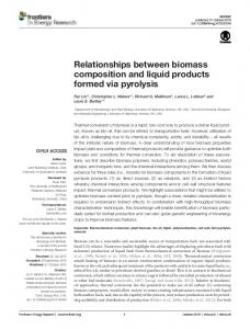
Figure 1.

Study area in the south-east USA for remote sensing of NDVI: North Carolina, South Carolina and Georgia.

ENSO and vegetation vigour

3079

that encompasses related changes in Paci c Ocean region sea level pressure and ‘disruption’ of atmospheric circulation patterns (Carleton 1998). Recognition of ENSO ‘events’—warm and cold SST phases, in addition to the normal state—has been based primarily on two diVerent indices: the Southern Oscillation Index (SOI ), usually calculated as the diVerence in Mean Sea Level Pressure (MSLP) anomalies between Tahiti and Darwin, Australia, and SSTs from various El Ninõ ‘sensitive’ regions of the equatorial Paci c Ocean (Allan et al. 1996 ). The four primary, documented El Ninõ sensitive regions of the Paci c Ocean have been dubbed regions Ninõ 1, Ninõ 2, Ninõ 3 and Ninõ 4 (Allan et al. 1996 ). Region Ninõ 3 (from 90° W to 150° W and from 5° N to 5° S) has been particularly prominent in recent ENSO research (Trenberth 1997). Recently, the Climate Prediction Center of the National Oceanic and Atmospheric Administration’s (NOAA) National Centers for Environmental Prediction has introduced a new SST index for an ENSO sensitive region named Ninõ 3.4 (from 120° W to 170° W and from 5° N to 5° S; gure 2), so named because it straddles regions Ninõ 3 and Ninõ 4 (Trenberth 1997). Trenberth (1997 ) proposes that the Ninõ 3.4 region is most sensitive to the initiation, duration, dissipation and magnitude of ENSO events. He uses this region to de ne ENSO warm and cold phases as ve month running mean SST anomalies of greater or lesser than 5° C, respectively. The SST signature of region Ninõ 3.4 from 1982 to 1992 is used in this study as an index of ENSO behaviour. 2.2. T he NDV I as a proxy for vegetation character The diVerence in re ectance at diVerent wavelengths of the electromagnetic spectrum for vegetated surfaces allows for the recognition of vegetation and vegetation character using satellite remote sensing. Vegetation typically re ects relatively weakly in the wavelengths of the visible band (VIS) compared to its strong re ectance in the near-infrared (NIR) wavelengths (Bannari et al. 1995 ). This property can be exploited to create an index that measures the diVerence between the re ectance of the two bands and that yields information about the vegetated surface. The NDVI is generally calculated as the following, most often using raw data from the MultiSpectral Scanner (MSS) or AVHRR aboard the Landsat and NOAA series of satellite platforms, respectively: (NIR reflectance VIS reflectance)/(NIR reflectance+VIS reflectance)

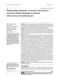
Figure 2.

(1)

Location of the ENSO sensitive region Ninõ 3.4: 120° W–170° W and 5° N–5° S.

3080

J. Mennis

The NDVI yields a value of between 1.0 and 1.0, with vegetated surfaces generally having values of between 0.1 and 0.7 (Carleton 1991 ). Non-vegetated surfaces typically have an NDVI value of less than 0.0 (they re ect slightly higher in the VIS than NIR wavelengths) . For vegetation, higher NDVI values correspond to an increase in vegetation ‘greenness’ or vigour, controlled by a combination of vegetation type, health, photosyntheti c activity and canopy density (Bannari et al. 1995, Lobo et al. 1997 ). Through time series analysis, interpretation of NDVI data has been extended to indicate land surface–climate interactions (Carleton et al. 1994, Carleton and O’Neal 1995), landscape change (Lambin 1996, Lambin and Ehrlich 1996), vegetation stress (e.g. drought ) (Nicholson et al. 1990) and phenology (Lobo et al. 1997 ). Because of the sensitivity of vegetation to climate, NDVI time series data can be reliable indicators of eco-climatologic variables such as temperature (Lobo et al. 1997, Yang et al. 1997 ) and precipitation, although these relationships are explicitly regional in nature. The temporal response of NDVI usually lags behind the uctuations of associated climate variables. Agricultural yields have also been successfully estimated using NDVI (Hayes and Decker 1996, Rasmussen 1998) and entered into predictive crop models (Moulin et al. 1998 ). Given the recent availability of homogeneous long term time series of NDVI data and the established precedent of NDVI-based monitoring of ‘natural’ and agricultural vegetation, NDVI is used in this study to capture vegetation character change over time. Caution, however, must be advised in interpreting the NDVI. The NDVI values are not only sensitive to vegetation characteristics but also to atmospheric variables, particularly the amount of water vapour and the presence of aerosols. NDVI data are also aVected by cloud contamination, sensor degradation, orbital drift, the anisotropic and transmissive radiation properties of plant canopies, and the in uence of moisture, colour and other soil properties (Halpert 1991, Pinty et al. 1993, Bannari et al. 1995 ). These data quality issues, and their speci c relation to the NDVI data used in the present study, are discussed in more depth in §3.1. 2.3. T racking the ENSO signal using NDV I Studies exploring the relationship of interannual uctuations of NDVI (or vegetation) with ENSO have focused primarily on Africa. Anyamba (1994) and Anyamba and Eastman (1996 ) use NDVI as a proxy for climate and apply principal components analysis (PCA) to extract and compare the various temporal signatures of NDVI with those of the SOI, Paci c Ocean SST and Paci c Ocean outgoing longwave radiation (OLR) for the years 1986 –1990. They noted that the SOI was signi cantly correlated with NDVI in southern Africa (r=0.65, signi cant at the 0.0001 level); ENSO warm phase events were associated with low NDVI values, due to decreased precipitation (Anyamba and Eastman 1996, p. 2542 ). These authors found that the correlation value did not signi cantly increase if the NDVI time series was ‘time lagged’, but stayed approximatel y constant up to a time lag of 2 months. Other interannual uctuations in NDVI were found for the Sahel and East Africa but were apparently not related to ENSO. Cane et al. (1994) used region Ninõ 3 SSTs to predict maize yield in Zimbabwe throughout the period 1970–1993 and found that greater than 60% of the variation in yield could be explained by the SST signature. They also found that correlation values declined only slightly when the maize yield was time lagged behind the SSTs by up to 10 months; at a time lag of greater than 10 months correlation values declined precipitously.


3081

Myneni et al. (1996) used monthly 1982–1990 NDVI data as a proxy for precipitation in their analysis of rainfall in arid and semi-arid areas of Africa, Australia and South America and their relation to region Ninõ 3 SSTs. These authors examined SST/NDVI correlation values on a pixel by pixel basis and demonstrate d that ENSO warm phase events were associated with lower than average rainfall in north-eastern Brazil and eastern Australia and higher than average rainfall in south-eastern South America. ENSO warm phase events were also found to have a strong association with climate in Africa in the eastern, south-eastern and central southern regions. In a study focusing on North America, Harrower (1998) compared the SOI and Paci c North America Index (PNA, an ENSO associated teleconnection concerning the phase and amplitude of the ridge-trough pattern over North America) with four diVerent eco-climatologic regimes in the USA at a variety of spatial and temporal aggregations . Results generally indicated a weak but discernible relationship between ENSO warm phase events and lower NDVI values throughout North America, with the strongest relationship evident in the Paci c Northwest region. 3. Data and methods 3.1. Data acquisition Both SST and NDVI data for the years 1982 –1992 were acquired from the Goddard Distributed Active Archive Center (DAAC 1998 ). The SST dataset was derived from a combination of in situ data gathered from ship and buoy observations and satellite observations from the AVHRR, situated on board the NOAA-7, NOAA-9, NOAA-11 and NOAA-14 polar orbiting platforms. The data were aggregated to a spatial resolution of 1° latitude by 1° longitude from the original satellite resolution of 1.1 km. The SST dataset is global in scope, with an applied land mask, and was temporally averaged to yield the monthly mean SST anomaly from the climatologic SST mean for the month (DAAC 1998). For a more detailed review of the SST dataset generation procedures the reader is referred to DAAC (1998 ), Reynolds and Smith (1995), McClain et al. (1985 ), Walton (1988) and Kidwell (1991 ). The NDVI dataset was derived from the Path nder AVHRR Land (PAL) programme and encompass North America (a water mask was applied) with a spatial resolution of 7.6 km. Daily images were used to create 10 day composite images using the maximum brightness technique in which the highest daily NDVI value recorded over a 10 day period for each pixel was retained (DAAC 1998 ). For a more detailed review of the NDVI dataset generation procedures see DAAC (1998), (1993a, b), Holben (1986) and Kidwell (1991). While the SST and PAL AVHRR datasets were pre-processed by NOAA to reduce data error prior to distribution, and the use of AVHRR data for studies of interannual variability in vegetation vigour and SST is well established (e.g. Carleton and O’Neal 1995, Anyamba and Eastman 1996, Hernandez-Guerra and Nykjaer 1997, Myneni et al. 1998), there remains some unresolved data quality issues associated with these datasets, including sensor degradation and orbital drift (Gutman 1999 ). Orbital drift results in the gradual shift of equator crossing times over the life of AVHRR-carrying NOAA satellites. Consequently, the sun–target geometry of the AVHRR sensor for any earth surface location is altered over time, introducing a temporal trend in the solar radiation data (and derived NDVI time series) that is not due to any actual environmental process (Gutman 1999 ). AVHRR-derived SST data are also aVected by orbital drift because it is the ocean ‘skin temperature’ in the thermal infrared (TIR) wavelengths that the AVHRR

3082

J. Mennis

‘measures’. This skin temperature changes rapidly according to the duration of solar heating and is also sensitive to uctuations in wind speed and evaporation (Privette et al. 1995). These eVects are reduced through the use of SST datasets in which satellite data are constrained using available conventional in situ observations of SST, as in the present study. Note also that orbital drift is much more problematic for studies of long term environmental trends than it is for studies of interannual climate variability and the impacts of these climate uctuations on vegetation (Gutman 1999), which are the focus of this study. Another AVHRR data quality issue concerns the ability of 10 day compositing to eVectively mitigate cloud contamination in the PAL dataset (Gutman and Ignatov 1996 ). While 30-day compositing may provide an improvement, it would also signi cantly reduce the temporal resolution of the NDVI data so that less than monthlong variations in vegetation vigour may be missed. Consider, however, that the PAL dataset is a spatial aggregation of the original AVHRR data from a pixel resolution of 1.1 km to a resolution of 7.6 km, which also serves to reduce cloud contamination. In this study, the PAL NDVI data were additionally aggregated both spatially and temporally (as described in the next section), further diminishing the eVects of cloud contamination. Land cover data were acquired from the US Environmental Protection Agency (EPA) (EPA 1998), although the data were originally created by the US Geological Survey (USGS). The EPA oVers the data over the Internet as individual 1:250 000 scale USGS ‘sheets’ formatted in ARC/INFO ( by Environmental Systems Research Institute, Inc.) polygon coverage format. Coverages that encompass the states of Georgia, North Carolina and South Carolina were downloaded and joined at their edges to form a seamless land cover data layer. The land cover information is derived from interpretation of high altitude aerial photography taken in the 1970s and 1980s and manually digitized onto 1:250 000 scale USGS base maps. The dataset is projected in Albers equal area projection with metre units. Land cover is categorized based on the two-stage hierarchical Anderson classi cation system (Anderson et al. 1976). The minimum size man-made feature digitized is 10 acres with a minimum width of 660 feet; the minimum size natural feature digitized is 40 acres with a minimum width of 1320 feet. For more information on the land cover data processing procedures the reader is referred to EPA (1998 ), USGS (1998), Anderson et al. (1976 ) and Mitchell et al. (1977 ). 3.2. Data manipulation and analysis The NDVI imagery was geo-recti ed to an ARC/INFO polygon coverage of the USA projected in the Albers equal area projection, the same projection as the land cover data, using the ERDAS Imagine image processing package. Geographic point locations identi able on both the NDVI imagery and the USA polygon coverage, such as the southern tip of lake Michigan and Cape Hatteras on the Outer Banks of North Carolina, were used in the geo-recti cation process. The land cover data were found to be prohibitively large (over 180 000 individual polygons) in terms of processing time when used for overlay with the NDVI data using a Sun Ultrasparc 25. In addition, the resolution of the land cover data was so much ner than that of the NDVI data that generalizing the land cover data did not compromise the integrity of the analysis. The land cover data were therefore converted to ARC/INFO grid format with a grid cell size equal to that of the NDVI


3083

data (7.6 km). This procedure assigns to a grid cell a single land cover value that is the spatial majority land cover within that cell. NDVI values were then averaged for each image for the following Andersonlevel land cover codes: 21 (croplands and pasture), 41 (deciduous forests) and 42 (evergreen forests). In addition, the NDVI mean of all land covers (the entire region) was calculated for Georgia, North Carolina and South Carolina. This procedure yielded a 10 day temporal resolution, 1982 –1992 mean NDVI time series of images for each land cover class and the region as a whole. Each image in the SST dataset was ‘clipped’ to region Ninõ 3.4 of the equatorial Paci c Ocean. A 1982–1992 monthly mean SST anomaly time series of the clipped images was created by nding the mean SST anomaly for each SST image. In addition, each image was queried for the percentage of SST grid cells with temperature anomaly values above the following thresholds: 0.4, 0.6, 0.8, 1.0, 1.5, 2.0, 3.0 and 4.0° C. The query results were used to form 1982 –1992 monthly time series for the percentage of cells above each of these threshold values. Because the SST and NDVI data have diVerent temporal resolutions (monthly and 10 day, respectively), linear interpolation was used to ‘expand’ the SST dataset so that it contained the same number of temporal observations as the NDVI dataset. The justi cation for this procedure is given by the relatively high thermal inertia of the oceans, which generally respond to forcing on time scales on the order of weeks to months and are not prone to sudden or rapid uctuation in temperature, especially in the lower latitudes (Allan et al. 1996, Carleton 1998). In order to extract the interannual relationships between ENSO and vegetation character in the south-east USA, it was necessary to remove the seasonal variation present within the SST and NDVI datasets. Figure 3 shows region Ninõ 3.4 SST anomalies and the mean NDVI for all land covers in Georgia, South Carolina and North Carolina for 1982 –1992 and demonstrate s that the seasonal signal swamps the interannual variation in the NDVI data. Two diVerent methods were used to extract the interannual NDVI signal for purposes of comparison. The rst method calculated an NDVI anomaly time series. A ‘baseline’ NDVI time series for each land cover was calculated by averaging the mean NDVI value for each time of year (36 values, or three per month) over the entire time period. The appropriate baseline value for each time of year was then subtracted from the NDVI mean for each image, resulting in an NDVI anomaly

Figure 3.

Region Ninõ 3.4 mean SST anomaly vs south-east USA mean NDVI, 1982–1992.

3084

J. Mennis

time series for each land cover class. The second method used a moving average to remove the intra-annual uctuation (and also to mitigate potential cloud contamination by ‘smoothing’ the NDVI data). A year-long centred moving average (36 images per year) was calculated for both the SST and NDVI datasets for each land cover class. 4.

Results and discussion Figure 4 presents the moving average time series of percentages of SST cells above the various threshold anomaly values. Only the 0.4, 1.0, 1.5 and 2.0° C thresholds are shown for graphic clarity. The 3.0 and 4.0° C thresholds have a peak at 1982 but are at (0%) throughout the remainder of the time period. While all the threshold values shown capture the ENSO warm phase events of 1982–1983, 1986 –1988 and 1991 –1992, and the cold phase events of 1984 –1985 and 1988–1989 (Trenberth 1997 ), only the 2.0° C threshold value time series diVerentiates between the relative strengths of each warm phase event. This is demonstrate d by the higher SST peak evident in the 1982 –1983 ENSO warm phase, regarded as the strongest warm phase this century prior to that of 1997 –1998 (Glantz 1996 ). The mean NDVI and SST anomaly time series are presented in gure 5. Although an interannual NDVI pattern is discernible, having peaks at approximatel y 1984,

Figure 4.

Percentage of region Ninõ 3.4 SST anomaly cells above certain threshold values, 1982–1992.

Figure 5.

Region Ninõ 3.4 mean SST anomaly vs south-east USA mean NDVI anomaly, 1982–1992.


3085

1988 and 1990, there is no coherent signal that appears to correspond to the SST anomaly signal. Note, however, that peaks in SST anomaly, both positive and negative, are associated with greater than normal variation in mean NDVI anomaly value over a short period of time. This is especially evident in the extreme NDVI anomaly variation during the SST anomaly low at the 1984 –1985 boundary. It is possible that the extreme NDVI anomaly values are the result of cloud contamination, although this would imply that the 10 day composite NDVI data covering all three states were cloud contaminate d enough to signi cantly lower the NDVI mean for the entire region. While perhaps an unlikely scenario, it is possible given the typical south-east USA climate responses to ENSO forcing, discussed below. Note that with the exception of the positive anomaly peak at the boundary of 1984–1985, all extreme NDVI anomalies are negative, consistent with cloud contamination. Another possible explanation for the extreme NDVI anomalies is the presence of volcanic aerosols in the atmosphere. The extreme negative NDVI anomalies in 1982 and 1991 are temporally coincident with the El Chichon eruption in Mexico and El Pinatubo eruption in the Philippines, respectively, both of which had an eVect on AVHRR NDVI values (Strong and Stowe 1993, Long and Stowe 1994 ). Table 1 presents the results of correlation tests performed on combinations of the diVerent measures of SST anomaly and diVerent NDVI anomaly time series for each land cover class. Correlation values are signi cant but relatively low, indicating that ENSO patterns and interannual vegetation uctuations are only weakly related to one another. The correlation values are uniformly negative, however, suggesting that ENSO warm phase events are associated with less vegetation vigour in the south-east USA. Yearly moving average NDVI means for three diVerent land covers are presented in gure 6. Note that the moving average technique has smoothed the NDVI time series so that the extreme negative and positive anomalies that were easily recognizable in the NDVI anomaly series are not present. All land cover types show peaks in 1984 and 1990 (up to 0.55) and low values in 1982, 1986 and 1992, with 1982 being the lowest (0.43). Generally, deciduous forests had the highest NDVI values, although the signal is often indistinguishable from that of evergreen forests. Croplands consistently had a lower NDVI value, although the time series signatures for all land cover classes were very similar in shape. The lower NDVI of croplands as compared with the other land covers is most Table 1.

Correlation values between diVerent south-east USA land cover mean NDVI anomalies and measures of SST anomalies in region Ninõ 3.4, 1982–1992. All correlation values are signi cant at the 0.01 level. Measures of SST anomaly cells in region Ninõ 3.4 (% >°C)

NDVI anomalies Croplands Deciduous Evergreen All land covers

% >0.4

Mean

0.22 0.23 0.21 0.23

0.18 0.18 0.17 0.18

% >0.6

0.21 0.22 0.20 0.22

% >0.8 0.22 0.23 0.22 0.23

% >1 0.23 0.24 0.22 0.24

% >1.5 0.25 0.25 0.23 0.26

% >2 0.25 0.26 0.24 0.26

% >3 0.24 0.25 0.24 0.23

% >4 0.24 0.25 0.25 0.24

3086

Figure 6.

J. Mennis

South-east USA moving average mean NDVI, 1982–1992: croplands, deciduous forests and evergreen forests.

likely associated with diVerences in fractional vegetation cover and Leaf Area Index (LAI) (Carlson and Ripley 1997). While it may seem counterintuitive that the croplands land cover has a noticeably lower NDVI value than the other land cover classes, note that nearly all land in the south-east USA is vegetated; even residential and commercial areas contain a signi cant amount of lawn and tree cover. Perhaps the diVerence in NDVI data ‘signature’ between croplands and other land covers is a result of the structure of row crops and orchards, which creates a generally sparser vegetation pattern and greater soil exposure than other vegetated land covers in the south-east USA. The NDVI/land cover results are broadly similar to those found by Carleton et al. (1994) in their strati cation of summertime NDVI by the same land cover classi cations in the Midwest USA, including the lower response of croplands as compared to other vegetated land covers. They nd that surface moisture and temperature stress play signi cant roles in in uencing summertime NDVI values. It follows that it is the interannual uctuation of these and other non-stationar y variables (i.e. precipitation as opposed to soil composition) that control the interannual uctuation of NDVI in the south-east USA. Yearly moving average mean NDVI values for the entire three state region throughout 1982 –1992 ranged between 0.43 and 0.53 with peaks in 1984 and 1990 and lower values in 1982, 1986 and 1992, with 1982 being by far the lowest value ( gure 7). This NDVI time series clearly indicates a negative relationship with mean SST anomalies over the same time period (r= 0.57, signi cant at the 0.01 level). Note that this correlation value is signi cantly higher than that calculated using the ‘baseline’ approach, most likely because of the removal of the extreme peaks and dips present in the NDVI anomaly time series and also the smoothing of the SST data. Yearly moving average SST anomalies ranged from 0.34 to 0.24, peaking in 1982, 1987 and 1992 (with 1982 slightly more pronounced ) and recording lows during 1985 –1986 and 1988. These interannual NDVI uctuations correspond loosely to the typical climatic responses to ENSO events in the south-east USA. ENSO warm phase events usually produce higher than average wintertime precipitation and lower than average temperatures in the south-east USA (Ropelewski and Halpert 1986, Carleton 1998), while cold phase events are associated with drier conditions and no signi cant change in


Figure 7.

3087

Region Ninõ 3.4 moving average mean SST anomaly vs south-east USA moving average mean NDVI, 1982–1992.

precipitation (Allan et al. 1996). These climatologic responses to ENSO are teleconnected via the PNA. During a typical ENSO warm phase, the wintertime sub-tropical jet (STJ) intensi es in response to the enhanced latitude temperature gradients induced by the higher SSTs in the central and eastern tropical Paci c Ocean. At the same time, the PNA pattern favours a low pressure trough over the south-east USA (Philander 1990). Alternatively, however, Ropelewski and Halpert (1986) proposed that the ENSO warm phase related anomalous climate conditions over the south-east USA are less in uenced by the PNA and are more a function of the increased equatorial Paci c Ocean convection associated with ENSO warm phase events. This increased convection activity produces anomalously strong westerlies in the Gulf of Mexico and increases the frequency of storms in the south-east USA region. Correlation tests between each of the moving average mean NDVI and SST anomaly time series are presented in table 2. All four land cover classes have their maximum correlation value with the percentage of SST cells above 2.0° C. This relationship is evidenced more clearly in gure 8 which shows correlation values climbing as the threshold SST anomaly value increases from 0.4 to 2.0° C, then descending as the threshold continues to increase to 4.0° C. Note also that the maximum diVerence between correlation values for each land cover class also occurs at the 2.0° C threshold measure. This is most likely due to the sensitivity of this Table 2.

Correlation values between diVerent south-east USA land cover moving average mean NDVI and measures of moving average SST anomalies in region Ninõ 3.4, 1982–1992. All correlation values are signi cant at the 0.01 level. Measures of SST anomaly cells in region 3.4 (% >°C)

NDVI mean Croplands Deciduous Evergreen All land covers

% >0.4

Mean

0.54 0.55 0.55 0.57

0.45 0.46 0.46 0.47

% >0.6

0.52 0.53 0.53 0.54

% >0.8 0.56 0.57 0.56 0.58

% >1 0.59 0.61 0.59 0.62

% >1.5 0.65 0.68 0.66 0.68

% >2 0.71 0.76 0.73 0.74

% >3 0.66 0.69 0.68 0.67

% >4 0.66 0.68 0.67 0.67

3088

J. Mennis

Figure 8. Correlation values between moving average mean NDVI for diVerent south-east US landcovers and the percentage of SST cells above certain threshold anomaly values in region Ninõ 3.4.

threshold to the magnitudes of diVerent ENSO events, as opposed to simply their presence, as discussed above and shown in gure 4. As further evidence of the ability of the 2.0° C SST anomaly threshold to capture diVerences in warm and cold phase intensity in the ENSO signal, gure 9 shows the 2.0° C threshold measure of SST anomalies plotted against the croplands mean NDVI. Note that there is not only a clear negative relationship between the two time series, but the magnitudes of the peaks and valleys of the NDVI re ect those of the SST anomaly measure. Correlation tests were also performed on the time-lagged NDVI means for each land cover class with the 2.0° C SST anomaly threshold series. New correlation tests were run for zero time lag through 6 months time lag ( gure 10). Surprisingly, no time lag increased the correlation value for any land cover class, although the simultaneous correlation values remained essentially unchanged as the NDVI was lagged up to 1 month. Following 1 month, correlation values declined gradually for all land cover classes, but at an increasing rate as the time lag increased. It is possible that a time lag is present but is suppressed by the year-long moving average technique

Figure 9.

Moving average mean NDVI for croplands in the south-east USA vs the percentage of region Ninõ 3.4 SST anomaly cells greater than 2.0, 1982–1992.


3089

Figure 10. Correlation values between time-lagged moving average mean NDVI for diVerent south-east USA landcovers and the percentage of SST anomaly cells greater than 2.0 in region Ninõ 3.4, 1982–1992.

used to extract the interannual variation. However, the results of this study are consistent with other ENSO/NDVI studies that also found no signi cant increase in correlation with time-lagged NDVI time series (Anyamba and Eastman 1996, Myneni et al. 1996, Harrower 1998). 5.

Conclusion This study found that there is a subtle, yet clearly recognizable, relationship between ENSO warm and cold phase events and interannual uctuations in vegetation vigour in the south-east USA. Warm phase events were associated with a decline in vegetation vigour while cold phase events were associated with an increase. ENSO patterns had the strongest correlation with variation in deciduous forests and a lesser correlation with variation in evergreen forests and croplands. The threshold SST anomaly method for measuring ENSO patterns was found to be an improvement over mean SST in correlation tests with NDVI. The signal associated with the percentage of SST cells above the 2° C temperature anomaly was found to be the most closely correlated with the vegetation signal. While this particular anomaly value may or may not represent a truly signi cant threshold in relation to ENSO or its eVects on regional climate and vegetation, this research demonstrate d the potential of the threshold approach for future studies of ENSO forcing on regional climate and vegetation. The diVerence in the strength of correlation derived between the baseline and moving average approaches to extracting interannual vegetation change is also enlightening. The baseline approach revealed that while vegetation does respond to ENSO, it is a weak in uence that is subservient to other, probably more local, factors. Signi cantly, the moving average approach yielded higher correlation values. While this approach has been criticized for in ating correlation scores as an artefact of the technique itself (Eklundh 1998), it was used by Trenberth (1997) to suppress intraseasonal variation in his analysis of region Ninõ 3.4 SST data, and this method serves a similar purpose here. It is justi ed because of the gradual and lengthy nature of both ENSO and the NDVI response to ENSO, both of which have periodicities of greater than a year (Anyamba and Eastman 1996). Because the moving average

3090

J. Mennis

technique ‘smooths’ the NDVI data time series signature, it suppresses outlier data values associated with contamination by clouds and atmospheric aerosols and brings out the interannual uctuations present in the data. Of course, it also suppresses extreme NDVI data values that may be meaningful in the context of vegetation dynamics. The relatively high and low correlation values associated with the moving average and baseline methods, respectively, indicate that while there is clearly a relationship between ENSO and vegetation vigour in the south-east USA, it is largely unpredictable for any given year. This unpredictability likely re ects the inconsistency of the climatic response to ENSO forcing in the south-east USA and the dominance of other factors in controlling vegetation vigour. Even if the climatic response is consistently colder and wetter, these conditions may have diVerent impacts on vegetation depending on their severity. Regardless, while the equatorial Paci c Ocean SST signal may be useful in predicting crop yields in regions more directly impacted by ENSO, this research indicates that the relationship between ENSO and vegetation variation in the south-east USA, as indicated by correlation, is too unpredictable to aid in crop yield forecasting. However, improvements in the analysis and the use of additional, more sophisticated, analytical techniques may yield more informative results. Uncertainties in the analysis concerning the integration of NDVI and land cover data include spatial registration, diVerence in scale and accuracy, and spatial and temporal data aggregation and generalization. The use of higher resolution NDVI data and correlation analysis on a pixel by pixel basis (as opposed to using the NDVI means for each land cover class) may produce more robust results and indicate place-based, as well as land cover class-based, vegetation variation. Other analytical methods, such as Fourier analysis and PCA, and the inclusion of regional climatologic data in the analysis, such as temperature and precipitation, may allow for more sophisticated extraction of ENSO and non-ENSO related patterns in the NDVI signature. Acknowledgments I would like to thank Andrew Carleton and the two anonymous reviewers for their helpful and constructive comments on an earlier draft of this paper. I would also like to thank Bill Easterling and Al Peters for encouraging this research, Amy GriYn for assisting with the data processing, and the Distributed Active Archive Center at the Goddard Space Flight Center for distribution of the SST and NDVI data. References Allan, R., Linsday, J., and Parker, D., 1996, El Ninõ Southern Oscillation and Climatic Variability (Collingwood, Australia: CSIRO). Anderson, J. R., Hardy, E. E., Roach, J. T., and Witmer, R. E., 1976, A land use and land cover classi cation system for use with remote sensor data. US Geological Survey Professional Paper, 964. Anyamba, A., 1994, Retrieval of ENSO signal from vegetation index data. Earth Observer, 6, 24–26. Anyamba, A., and Eastman, J. R., 1996, Interannual variability of NDVI over Africa and its relation to El Nino/Southern Oscillation. International Journal of Remote Sensing, 17, 2533–2548. Bannari, A., Morin, D., and Bonn, F., 1995, A review of vegetation indices. Remote Sensing Reviews, 13, 95–120.


3091

Cane, M. A., Eshel, G., and Buckland, R. W., 1994, Forecasting Zimbabwean maize yield using eastern equatorial Paci c sea surface temperature. Nature, 370, 204–205. Carleton, A., 1991, Satellite Remote Sensing in Climatology (Bellhaven Press: London). Carleton, A. M., 1998, Ocean–atmosphere interactions. In Encyclopedia of Environmental Analysis and Remediation, edited by R. A. Meyers (New York: Wiley), pp. 3151–3188. Carleton, A. M., and O’Neal, M. O., 1995, Satellite-derived land surface climate ‘signal’ for the Midwest USA. International Journal of Remote Sensing, 16, 3195–3202. Carleton, A. M., Travis, D., Arnold, D., and Brinegar, R., 1994, Climatic-scale vegetation– cloud interactions during drought using satellite data. International Journal of Climatology, 14, 593–623. Carlson, T. N., and Ripley, D. A., 1997, On the relation between NDVI, fractional vegetation cover, and leaf area index. Remote Sensing of Environment, 62, 241– 252. DAAC, 1998, Distributed Active Archive Center web site. http://daac.gsfc.nasa.gov. Eklundh, L., 1998, Estimating relations between AVHRR NDVI and rainfall in East Africa at 10-day and monthly time scales. International Journal of Remote Sensing, 19, 563–568. EPA, 1998, US Environmental Protection Agency web site. http://www.epa.gov. Glantz, M. H., 1996, Currents of Change: El Nino’s Impact on Climate and Society (Cambridge, UK: Cambridge University Press). Gutman, G. G., 1999, On the use of long-term global data of land re ectances and vegetation indices derived from the advanced very high resolution radiometer. Journal of Geophysical Research, 104, 6241–6255. Gutman, G., and Ignatov, A., 1996, The relative merit of cloud/clear identi cation in the NOAA/NASA Path nder AVHRR Land 10-day composites. International Journal of Remote Sensing, 17, 3295–3304. Halpert, M. S., 1991, Climate monitoring using an AVHRR-based vegetation index. Palaeogeography, Palaeoclimatology, Palaeoecology, 90, 201–205. Harrower, M., 1998, Using the NDVI to study inter-annual climate variability in North America. M.S. paper, The Pennsylvania State University, University Park, PA. Hayes, M. J., and Decker, W. L., 1996, Using NOAA AVHRR data to estimate maize production in the United States corn belt. International Journal of Remote Sensing, 17, 3189–3200. Hernandez-Guerra, A., and Nykjaer, L., 1997, Sea surface temperature variability oV northwest Africa: 1981–1989. International Journal of Remote Sensing, 18, 2539–2558. Holben, B. N., 1986, Characteristics of maximum-value composite images from temporal AVHRR data. International Journal of Remote Sensing, 7, 1417–1434. Kidwell, K., 1991, NOAA Polar Orbiter Data User’s Guide. National Climatic Data Center, Washington, DC. Lambin, E. F., 1996, Change detection at multiple temporal scales: seasonal and annual variations in landscape variables. Photogrammetric Engineering and Remote Sensing, 62, 931–938. Lambin, E. F., and Ehrlich, D., 1996, The surface temperature–vegetation index space for land cover and land-cover change analysis. International Journal of Remote Sensing, 17, 463–487. Lobo, A., Marti, J. J. I., and Gimenez-Cassina, C. C., 1997, Regional scale hierarchical classi cation of temporal series of AVHRR vegetation index. International Journal of Remote Sensing, 18, 3167–3193. Long, C. S., and Stowe, L. L., 1994, Using the NOAA/AVHRR to study stratospheric aerosol optical thickness following the Mt. Pinatubo eruption. Geophysical Research L etters, 21, 2215–1128. McClain, E. P., Pichel, W. G., and Walton, C. C., 1985, Comparative performance of AVHRR-based multichannel sea surface temperature. Journal of Geophysical Research, 90, 11585–11601. Mitchell, W. B., Guptill, S. C., Anderson, K. E., Fegeas, R. G., and Hallam, C. A., 1977, GIRAS—A Geographic Information and Analysis System for Handling L and Use and L and Cover Data. U.S. Geological Survey, Reston, VA. Moulin, S., Bondeau, A., and Delecolle, R., 1998, Combining agricultural crop models and satellite observations: from eld to regional scales. International Journal of Remote Sensing, 19, 1021–1036.

3092


Myneni, R. B., Los, S. O., and Tucker, C. J., 1996, Satellite-based identi cation of linked vegetation index and sea surface temperature anomaly areas from 1982–1990 for Africa, Australia and South America. Geophysical Research L etters, 23, 729–732. Myneni, R. B., Tucker, C. J., Asrar, G., and Keeling, C. D., 1998, Interannual variations in satellite-sensed vegetation index data from 1981 to 1991. Journal of Geophysical Research, 103, 6145–6160. Nicholson, S. E., Davenport, M. L., and Malo, A. R., 1990, A comparison of the vegetation response to rainfall in the Sahel and east Africa, using normalized diVerence vegetation index from NOAA AVHRR. Climatic Change, 17, 209–241. Philander, S. G., 1990, El Ninõ, L a Ninã, and the Southern Oscillation (San Diego: Academic Press). Pinty, B., Leprieur, C., and Verstraete, M. M., 1993, Towards a quantitative interpretation of vegetation indices: part 1: biophysical canopy properties and classical indices. Remote Sensing Reviews, 7, 127–150. Privette, J. L., Fowler, C., Wick, G. A., Baldwin, D., and Emery, W. J., 1995, EVects of orbital drift on advanced very high resolution radiometer products: normalized diVerence vegetation index and sea surface temperature. Remote Sensing of Environment, 53, 164–171. Rao, C. R. N., 1993a, Degradation of the visible and near-infrared channels of the Advanced Very High Resolution Radiometer on the NOAAP9 spacecraft: assessment and recommendations for corrections. NOAA/NESDIS, Washington, DC. Rao, C. R. N., 1993b, Nonlinearity corrections for the thermal infrared channels of the Advanced Very High Resolution Radiometer: assessment and recommendations. NOAA/NESDIS, Washington, DC. Rasmussen, M. S., 1998, Developing simple, operational, consistent NDVI-vegetation models by applying environmental and climatic information. Part II: Crop yield assessment. International Journal of Remote Sensing, 19, 119–139. Reynolds, R. W., and Smith, T. M., 1995, A high-resolution global sea surface temperature climatology. Journal of Climate, 8, 1571–1583. Ropelewski, C. F., and Halpert, M. S., 1986, North American precipitation and temperature patterns associated with the El Nino/Southern Oscillation (ENSO). Monthly Weather Review, 114, 2352–2362. Ropelewski, C. F., and Halpert, M. S., 1987, Global and regional scale precipitation patterns associated with the El Ninõ/Southern Oscillation. Monthly Weather Review, 115, 1606–1626. Strong, A. E., and Stowe, L. L., 1993, Comparing aerosols from El Chicon and Mount Pinatubo using AVHRR data. Geophysical Research L etters, 20, 1183–1186. Trenberth, K. E., 1997, The de nition of El Nino. Bulletin of the American Meteorological Society, 78, 2771–2777. USGS, 1998, US Geological Survey web site. http://www.usgs.gov. Walton, C. C., 1988, Nonlinear mulitchannel algorithms for estimating sea surface temperature with AVHRR satellite data. Journal of Applied Meteorology, 27, 115–124. Yang, W., Yang, L., and Merchant, W., 1997, An assessment of AVHRR/NDVI-ecoclimatological relations in Nebraska, U.S.A. International Journal of Remote Sensing, 18, 2161–2180.