EXPLORING THE TREE OF NUMERICAL SEMIGROUPS

arXiv:1305.3831v1 [math.CO] 16 May 2013

EXPLORING THE TREE OF NUMERICAL SEMIGROUPS JEAN FROMENTIN Abstract. In this paper we describe an algorithm visiting all the numerical semigroups up to a given genus using a new representation of numerical semigroups.

1. Introduction A numerical semigroup S is a subset of N containing 0, close under addition and of finite complement in N. For example the set SE = {0, 3, 6, 7, 9, 10} ∪ [12, +∞[

(1)

is a numerical semigroup. The genus of a numerical semigroup S, denoted by g(S), is the cardinality of N \ S, i.e, g(S) = card(N \ S). For example the genus of SE defined in (1) is 6, the cardinality of {1, 2, 4, 5, 8, 11} For a given positive integer g, the number of numerical semigroups is finite and is denoted by ng . In J.A. Sloane’s on-line encyclopedia of integer [1] we find the values of ng for g 6 52. These values have been obtain by M. Bras-Amor´ os (view [2] for more details for g 6 50). On his home page [3], M. Delgado gives the value of n55 without specifying the values of n53 and n54 . M. -Bras Amor´ os used a depth first search exploration of the tree of numerical semigroups up to a given genus. This tree was introduced by J.C. Rosales and al. in [4] and it is the subject of the Section 2. Starting with all the numerical semigroups of genus 49 she obtained the number of numerical semigroups of genus 50 in 18 days on a pentium D runing at 3GHz. In the package NumericalSgs [5] of GAP [6], M. Delgado together with P.A. Garcia-Sanchez and J. Morais used the same method of exploration. The paper is divided as follows. In section 2 we describe the tree of numerical semigroups and give bounds for some parameters attached to a numerical semigroup. In Section 3 we describe a new representation of numerical semigroups that is well suited to the construction of the tree. In Section 4 we describe an algorithm based on the representation given in Section 3 and give its complexity. Section 5 is more technical, and is devoted to the optimisation of the algorithm introduced in Section 4. 2. The tree of numerical semigroups We first start by some notations. 1

2

JEAN FROMENTIN

Definition 2.1. Let S be a numerical semigroup. We define i) m(S) = min(S \ {0}), the multiplicity of S; ii) g(S) = card(N \ S), the genus of S; iii) c(S) = 1 + max(N \ S), the conductor of S for S different from N. By convention the conductor of N is 0. By definition a numerical semigroup is an infinite object. We need a finite description of such a semigroup. That is the role of generating sets. Definition 2.2. A subset X of a semigroup is a generating set of S if every element of S can be express as a sum of elements in X. Notation 2.3. A numerical semigroup admitting X = {x1 < x2 < ... < xn } as generating set is denoted by S = hx1 , ..., xℓ i. We now introduce a specific generating set. Definition 2.4. A non-zero element x of a numerical semigroup S is said to be irreducible if it cannot be expressed as a sum of two non-zeros elements of S. We denote by Irr(S) the set of all irreducible elements of S. Proposition 2.5. Let S be a numerical semigroup. Then Irr(S) is the minimal generating set of S. Proof. Assume for a contradiction, that there exists an integer x in S than cannot be decomposed as a sum of irreducible elements. We may assume that x is minimal with this property. As x cannot be irreducible, there exist y and z in S \ {0} satisfying x = y + z. Since we have y < x and z < x, the integers y and z can be expressed as a sum of irreducible elements of S and so x = y + z is a sum of irreducible elements, in contradiction to hypothesis. As irreducible elements of S cannot be decomposed as the sum of two non-zeros integers in S, they must occur in each generating set of S.  We recall that Ap´ery elements of a numerical semigroup S associated to m(S) are the integers x in S such that x−m(S) is no longer in S. We denote by App(S) the set of these elements. It is well known that the cardinality of App(S) is exactly m(S) (see [7] for example). Note that the set Irr(S) is in included in App(S). In particular, the set Irr(S) is finite and its cardinality is at most m(S). If we reconsider the numerical semigroup of (1), we obtain SE = {0, 3, 6, 7, 9, 10} ∪ [12, +∞[= h3, 7i

(2)

Let S be a numerical semigroup. The set T = S ∪ {c(S) − 1} is also a numerical semigroup and its genus is g(S) − 1. As [c(S) − 1, +∞[ is included in T we have c(T ) 6 c(S) − 1. Therefore every semigroup S of genus g can be obtained from a semigroup T of genus g − 1 by removing an element of T greater than or equal to c(T ). Proposition 2.6. Let S be a numerical semigroup and x an element of S. The set S x = S \ {x} is a numerical semigroup if and only if x is irreducible in S.

EXPLORING THE TREE OF NUMERICAL SEMIGROUPS

3

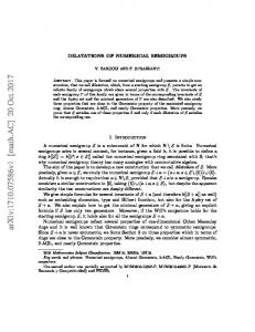
Proof. If x is not irreducible in S, then there exist a and b in S \ 0 such that x = a + b. Since a 6= 0 and b 6= 0 hold, the integers a and b belong to S \ {x}. Since x = a + b and x 6∈ S x , it follows that S x is not stable under addition. Conversely, assume that x is irreducible in S. As 0 is never irreducible, the set S x contains 0. Let a and b be two integers belonging to S x . The set S is stable under addition, hence a + b lies in S. As S is equal to S x ∪ {x}, the integer a + b also lies in S x except if it is equal to x. The latter is impossible since a and b are different from x and x is irreducible.  Proposition 2.6 implies that every semigroup T of genus g can be obtained from a semigroup S by removing a generator x of S that is greater than c(S). Hence relations T = S x = S \ {x} hold. We construct the tree of numerical semigroups, denoted by T as follows. The root of the tree is the unique semigroup of genus 0, i.e, h1i that is equal to N. If S is a semigroup in the tree, the sons of S are exactly the semigroup S x where x belongs to Irr(S) ∩ [c(s), +∞[. By convention, when depicting the tree, the ,numerical semigroup S x is in the left of S y if x is smaller than y. The above remarks imply that a semigroup S has depth g in mathcalT if and only if its genus is g, see Figure 1. We denote by T 6g the subtree of T resticted to all semigroup of genus 6 g. As the reader can check, the main difficulty to characterize the sond of a semigroup is to determine its irreducible elements. In [5], the semigroup are given by their Ap´ery set App(S) and then the main difficulty is to describe App(Sx ) from App(S). This approach is elegant but not sufficiently basic for our optimisations. We conclude this section with some basic results on numerical semigroups of a given genus. Let S be a numerical semigroup. We first prove : x ∈ Irr(S) implies

x 6 c(S) + m(S).

(3)

If y is a positive integer with y > c(S) + m(S) then y lies in S (as y > c(S) holds). Moreover, we always have y−m(S) > c(s) and so y is not irreducible. As N \ S contains {1, .., m(S) − 1} we have m(S) 6 g(S) + 1.

(4)

Let x be an element of S ∩ [0, c(S) − 1]. The integer y = c(S) − 1 − x lies in [0, c(S) − 1]. Moreover y is not in S, for otherwise we write c(S) − 1 = y + x where x, y are elements of S implying c(S) − 1 ∈ S. In contradiction with the definition of conductor. Thus we define an involution ψ : [0, c(S) − 1] → [0, c(S) − 1] x 7→ c(S) − 1 − x that send S ∩ [0, c(S) − 1] into [0, c(S) − 1] \ S. The cardinality of [0, c(S)[\S is exactly g(S). Let us denote by k the cardinality of S ∩ [0, c(S) − 1]. Since ψ is injective we must have k 6 g(S). From the relation [0, c(S)[= S ∩ [0, c(S)[⊔[0, c(S)[\S

4

JEAN FROMENTIN

h1i 1 h2, 3i 2

3

h3, 4, 5i 3

4

h4, 5, 6, 7i 4

5

6

h2, 5i 5 h3, 5, 7i

7

5

5 h3, 4i

h2, 7i

7

h5, 6, 7, 8, 9i h4, 6, 7, 9i h4, 5, 7i h4, 5, 6i h3, 7, 8i h3, 5i

7 h2, 9i

Figure 1. The first five layers of the tree T of numerical semigroups, corresponding to T 65 . A generator of a semigroup is in gray if it is not in [c(S), +∞[. An edge between a semigroup S and its son S ′ is labelled by x is S ′ is obtained from S by removing x, that is S ′ = S x . we obtain c(S) = k + g(S) and so c(S) 6 2g(S).

(5)

3. Decomposition number The aim of this section is to describe a new representation of numerical semigroups. which is well suited to a efficient exploration of the tree T of numerical semigroups. Definition 3.1. Let S be a numerical semigroup. For every x of N we set DS (x) = {y ∈ S | x − y ∈ S and 2y 6 x} and dS (x) = card DS (x). We called dS (x) the S-decomposition number of x. The application dS : N → N is the S-decomposition numbers function. Assume that y is an element of DS (x). By very definition of DS (x), the integer z = x − y also belongs to S. Then x can be decomposed as x = y + z with y and z in S. Moreover the condition 2y 6 x implies y 6 z. In other words if we define DS′ (x) to be the set of all (y, z) ∈ S × S with x = y + z and y 6 z then DS (x) is the image of DS′ (x) under the projection on the

EXPLORING THE TREE OF NUMERICAL SEMIGROUPS

5

first coordinate. Hence DS (x) describes how x can be decomposed as sums of two elements of S,-. This is why dS (x) is called the S-decomposition number of x. Example 3.2. Reconsider the semigroup SE given at (1). The integer 14 admits three decompositions as sums of two elements of S, namely 14 = 0 + 14, 14 = 3 + 11 and 14 = 7 + 7. Thus the set DSE (14) is equal to {0, 3, 7} and dSE equals 3. Lemma 3.3. For jevery numerical semigroup S and every integer x ∈ N, we xk and the equality holds for S = N. have dS (x) 6 1 + 2  x Proof.  x As the set DS (x) is included in {0, ..., 2 }, the relation dS (x) 6 1 + 2 holds. For S = N we have the equality for DS (x) and so for dS (x).  Proposition 3.4. Let S be a numerical semigroup and x ∈ N \ {0}. We have: i) x lies in S if and only if dS (x) > 0. ii) x is in Irr(S) if and only if dS (x) = 1. Proof. We start with i). If x is an element of S then x equals 0 + x. The relation 2 × 0 6 x and 0 ∈ S imply that DS (x) contains 0, and so dS (x) > 0 holds. Conversely, the relation dS (x) > 0 implies that DS (x) is non-empty. Let y be an element of DS (x). As y and x − y belong to S, by definition, the integer x = (x − y) + y is in S (since S is stable by addition). Let us show ii). Assume x is irreducible in S. There cannot exist y and z in (S \ {0})2 such that x = y + z. The only possible decomposition of x as a sum of two elements of S is x = 0 + x. Hence, the set DS (x) is equal to {0} and we have dS (x) = 1. Conversely, let x such that dS (x) = 1. By i) the integer x must be in S. As x = 0 + x is always a decomposition of x as a sum of two elements in S, we obtain DS (x) = {0}. If there exist y and z in S such that y 6 z and x = y + z hold then y lies in DS (x). This implies y = 0 and z = x. Hence x is irreducible in S.  We note that 0 is never irreducible despite the fact dS (0) is 1 for all numerical semigroup S. We now explain how to compute the S-decomposition numbers function of a numerical semigroup from these of its father. Proposition 3.5. Let S be a numerical semigroup and x be an irreducible element of S. Then for all y ∈ N \ {0} we have ( dS (y) − 1 if y > x and dS (y − x) > 0, dS x (y) = dS (y) otherwise. Proof. Let y be in N \ {0}. We have DS x (y) = {z ∈ S x | y − z ∈ S x and 2z 6 y}

6

JEAN FROMENTIN

and DS x (y) is a subset of DS (y). We have DS (y) \ DS x (y) = E ⊔ F where ( {x} if y − x ∈ S x and 2x 6 y, E= ∅ otherwise. F = {z ∈ S | y − z = x and 2z 6 y} Since the relation y −x ∈ S x can be rewritten as the conjunction of y −x ∈ S and y 6= 2x, we obtain ( {x} if y − x ∈ S and 2x < y, E= ∅ otherwise. By Proposition 3.4, the relation y − x ∈ S is equivalent to y > x and dS (y − x) > 0, we have ( {x} if y > x and dS (y − x) > 0 and 2x < y, E= ∅ otherwise. On the other hand, we have F = {z ∈ S | y − z = x and 2z 6 y} = {z ∈ S | z = y − x and y 6 2x} ( {y − x} if y − x ∈ S and y 6 2x, = ∅ otherwise. As in the case of E, we get ( {y − x} if y > x and dS (y − x) > 0 and y 6 2x, F = ∅ otherwise. In E we have the constraint 2x < y while in F we have y 6 2x, hence only one of the sets E or F can be non-empty. This implies   if y > x and dS (y − x) > 0 and y 6 2x, {x} x DS (y) \ DS (y) = {y − x} if y > x and dS (y − x) > 0 and y > 2x,   ∅ otherwise. Therefore we obtain

( dS (y) − 1 dS x (y) = dS (y)

if y > x and dS (y − x) > 0, otherwise. 

4. A new algorithm We can easily explore the tree of numerical semigroups up to a genus G using a depth search first algorithm using a stack (see 1). This approach does not seem to have been used before. In particular, M. Bras-Amor´ os and M. Delgado use instead a breadth search first exploration. The main

EXPLORING THE TREE OF NUMERICAL SEMIGROUPS

7

advantage in our approach is the small memory needs. The cost to pay is that, if we want to explore the tree deepero, we must restart from the root. Algorithm 1 Depth search first exploration of the tree of numerical semigroups 1: 2: 3: 4: 5: 6: 7: 8: 9: 10: 11: 12: 13: 14: 15:

procedure Explore(G) Stack stack S ← h1i while stack is not empty do S ← stack.top() stack.pop() if g(S) < G then for x from c(S) to c(S) + m(S) do if x ∈ Irr(S) then S.push(Sx ) end if end for end if end while end procedure

⊲ the empty stack

In Algorithm 1 we do not specify how to compute c(S), g(S) and m(S) from S neither how to test if an integer is irreducible. It also miss the characterisation of S x from S. These items depend heavily of the representation of S. Our choice is to use the S-decomposition numbers function. The first task is to use a finite set of such numbers to characterise the whole semigroup. Proposition 4.1. Let G be an integer and S be a numerical semigroup of genus g 6 G. Then S is entirely described by δS = (dS (0), ..., dS (3 G)). More precisely we can obtain c(S), g(S), m(S) and Irr(S) from δS . Proof. By (5) we have c(S) 6 g(S) and so the S-decomposition number of c(S) occurs in δS . Since c(S) is equal to max(N \ S), Proposition 4.1 implies c(S) = 1 + max{i ∈ [0, ..., 3G], dS (i) = 0}. As all elements of N\S are smaller than c(S), their S-decomposition numbers are in δS and we obtain g(S) = card{i ∈ [0, .., 3G], dS (i) = 0}. By (4) the relation m(S) 6 g(S) + 1 holds. This implies that the Sdecomposition number of m(S) appears in δS : m(S) = min{i ∈ [0, ..., 3G], dS (i) > 0}. Since, by (3), all irreducible elements are smaller than c(S) + m(S) − 1, which is itself smaller than 3G, equations (4) and (5) give Irr(S) = {i ∈ [0, ..., 3G], dS (i) = 1}.

8

JEAN FROMENTIN

 Even though it is quite simple, the computation of c(S), m(S) and g(S) from δS has a non negligible cost. We represent a numerical semigroup S of genus g 6 G by (c(S), g(S), c(S), δS ). In an algorithmic context, if the variable S stands for a numerical semigroup we use: – S.c, S.g and S.m for the integers c(S), g(S) and m(S); – S.d[i] for the integer dS (i). For example the following Algorithm initializes a representation of the semigroup N ready for an exploration up to genus G. Algorithm 2 Return the root of T for an exploration up to genus G function Root(G) R.c ← 1 R.g ← 0 R.m ← 1 for x from 1 to 3 G do  R.d[x]← 1 + 2x end for return R end function

⊲ R stands for N

We can now describe an algorithm that returns the representation of the semigroup S x from that of the semigroup S where x is an irreducible element of S greater than c(S). Algorithm 3 Returns the son Sx of S with x ∈ Irr(S) ∩ [c(S), c(S) + m(S)[. 1: 2: 3: 4: 5: 6: 7: 8: 9: 10: 11: 12: 13: 14: 15: 16:

function Son(S,x,G) T.c ← x + 1 T.g ← S.g + 1 if x > S.m then T.M ← S.m else T.M ← S.m + 1 end if T.d ← S.d for y from x to 3 G do if S.d[y − x] > 0 then T.d[y] ← T.d[y] − 1 end if end for return T end function

⊲ T stands for Sx

EXPLORING THE TREE OF NUMERICAL SEMIGROUPS

9

Proposition 4.2. Running on (S, x, G) with g(S) 6 G, x ∈ Irr(S) and x 6 c(S), Algorithm 3 returns the numerical semigroup Sx in time O(log(G)×G). Proof. By construction S x is the semigroup S \ {x}. Thus the genus S x is g(S) + 1, see Line 1. Every integer of I = [x + 1, +∞[ lies in S since x is greater than c(S), so the interval I is included in S x . As x does not belong to S, the conductor of S x is x+1, see Line 2. For the multiplicity of S x we have two cases. First, if x > m(S) holds then m(S) is also in S x and so m(S x ) is equal to m(S). Assume now x = m(S). The relation x(S) > c(S) and the characterisation of m(S) implies x = m(S) = c(S). Thus S x contains m(S) + 1 which is m(S x ). The initialisation of m(S x ) is done by Lines 4 to 8. The correctness of the computation of δS x (see Proposition 4.1) done from Line 9 to Line 15 is a direct consequence of Proposition 3.4. Let us now prove the complexity statement. Since by (5) and (4) we have x 6 3G together with m(S) 6 G + 1, each line from 2 to 8 is done in time O(log(G)). The for loop needs O(G) steps and each step is done in time O(log(G)). Summarizing, these results give that the algorithm runs in time O(log(G) × G).  Algorithm 4 Returns an array containing the value of ng for g 6 G 1: 2: 3: 4: 5: 6: 7: 8: 9: 10: 11: 12: 13: 14: 15: 16: 17: 18:

function Count(G) n ← [0, ..., 0] ⊲ n[g] stands for ng and is initialised to 0 Stack stack ⊲ the empty stack S ← Root(G) while stack is not empty do S ← stack.top() stack.pop() n[S.g] ← n[S.g] + 1 if S.g < G then for x from S.c to S.c + S.m do if S.d[x] = 1 then S.push(Son(S, x, G)) end if end for end if end while return n end function

Proposition 4.3. Running on G ∈ N, Algorithm Count returns the array [n0 , ..., nG ] in time   G X ng  O log(G) × G × g=0

10

JEAN FROMENTIN

and its space complexity is O(log(G) × G3 ). Proof. The correctness of the algorithm is a consequence of Proposition 4.2 and of the description of the tree T of numerical semigroups. For the time complexity, let us remark that Algorithm Son is called for every semigroup of the tree T 6G (the restriction of T to semigroup of genus P 6 G). Since there are exactly N = G g=0 ng such semigroups, the time complexity of Son established in Proposition 4.2 guarantees that the running time of Count is in O(log(G) × G × N ), as stated. Let us now prove the space complexity statement. For this we need to describe the stack through the run of the algorithm. Since the stack is filled with a depth first search algorithm, it has two properties. The first one is that reading the stack from the bottom to the top, the genus of semigroup increases. The second one is that, for all g ∈ [0, G], every semigroup of genus g in the stack has the same father. As the number of sons of a semigroup S is the number of S-irreducible elements in [c(S), c(S) + m(S) − 1], a semigroup S has at most m(S) sons. By (4), this implies that a semigroup of genus g as at most g + 1 sons. Therefore the stack contains at most g + 1 semigroup of genus g + 1 for g 6 G. So the size of the stack is bounded by S=

G X g=0

g=

G(G + 1) 2

A semigroup is represented by a quadruple (c(S), g(S), m(S), δS ). By equations (5) and (4), we have c 6 2g(S) and m 6 g(S) + 1. As g(S) 6 G holds, the integers c, g and m of the representation of S require a memory space in O(log(G)). The size of δS = (dS (0), ..., dS (3G)) is exactly 3G + 1. Each entry of δS is the S-decomposition number of an integer smaller than 3G and hence requires log(G) bytes of memory space. Therefore the space complexity of δS is in O(log(G) × G), which implies that the space complexity of the Count algorithm is O(log(G) × G × S) = O(log(G) × G3 ).  5. Technical optimizations and results Assume for example that we want to construct the tree T 6100 of all numerical semigroup of genus smaller than 100. In this case, the representation of numerical semigroup given in Section 3 uses decomposition numbers of integers smaller than 300. By Lemma 3.3, such a decomposition number is smaller than 151 and requires 1 byte of memory. Thus at each for step of Algorithm Son, the CPU actually works on 1 byte. However current CPUs work on 8 bytes. The first optimization uses this point. To go further we must specify that the array of decomposition numbers in the representation of a semigroup corresponds to consecutive bytes in memory. In the for loop of Algorithm Son we may imagine two cursors:

EXPLORING THE TREE OF NUMERICAL SEMIGROUPS

11

the first one, denoted src pointing to the memory byte of S.d[0] and the second one, denoted dst pointing to the memory byte T.d[y]. Using these two cursors, Lines 10 to 14 of Algorithm Son can be rewritten as follows src ← address(S.d[0]) dst ← address(T.d[x]) i←0 while i 6 3G − x do if content(src) > 0 then decrease content(dst) by 1 end if increase src,dst,i by 1 end while In this version we can see that the cursors src and dst move at the same time and that the modification of the value pointed by dst only needs to access the values pointed by src and dst. We can therefore work in multiple entries at the same time without collision. Current CPUs allow this thanks to the SIMD technologies as MMX, SSE, etc. The acronym SIMD stands for Single Operation Multiple Data. The MMX technology permits to work on 8 bytes in parallel while the SSE works in 16 bytes. As the rest of the CPU works on 8 bytes, the SSE technology needs some constraint on memory access than cannot be fulfilled in our algorithm. This motivate our choice to use the MMX technology. More precisely, we use three commands: pcmpeqb, pandn and psubb. These commands work on two arrays of 8 bytes, called s and d here. In each case the array d is modified. We denote bytes by {0, 1}-words of length 8. After a call to pcmpeqb(s,d) the ith entry of d contains 11111111 if s[i] = d[i] holds and 00000000 otherwise. The command pand(s,d) store in d[i] the value of the byte-logic operation s[i] and (not d[i]). When pand(s,d) is called the new value of d[i] is s[i] − d[i]. Glueing all the pieces together we obtain the following version of the for loop of Algorithm Son : 1: src ← address(S.d[0]) 2: dst ← address(T.d[x]) 3: i ← 0 4: while i 6 3G − x do 5: t ← [00000000, ..., 00000000] ⊲ 8 bytes equal to 00000000 6: pcmpeqb(src,t) 7: pandn([00000001,...,00000001],t) 8: psub(dst,t) 9: dst ← t ⊲ copy the array [t[0], ..., t[7]] to [d[0], ..., d[7]] 10: increase src,dst,i by 8 11: end while

12

JEAN FROMENTIN

Let us explain how this works in more details. Let i be an integer in {0, ..., 7}. After Line 5, the value of t[i] is 0000000. After Line 6, we have ( 11111111 if src[i] = 00000000 (corresponding to 0) t[i] = 00000000 otherwise Line 7 performs a logical and between 00000001 and not t[i]. Hence the result byte is 00000001 if the last byte of t[i] is 0 and 00000000 otherwise: ( 00000000 if src[i] = 00000000 (corresponding to 0) t[i] = 00000001 otherwise Line 8 subtracts t[i] (which is equal to 0 or 1) from dst[i] according to Proposition 2.6. Finally we shift the cursor src and dst by eight cases. Our second optimization is to use parallelism on exploration of the tree. Today, CPU of personal computer have several cores (2, 4 or more). The given version of our exploration algorithm uses a single core and so a fraction only of the power of a CPU. Our method of parallelism is very simple: for G ∈ N, we cut the tree T 6G in sub-trees T1 , ..., Tn and we launch our algorithm on these sub-trees. The advantage of this method is that there is no communication between the instances of our algorithm. The disadvantage is that the cutting controls the efficiency of the parallelism. Assume for example that we want to explore the tree T 640 . We first determine all numerical semigroups S1 , ...Sn20 of genus 20. To explore T it remains to explore the tree Ti rooted in Si for i = 1, ..., n20 . This works but the time to explore T1 is similar to the time need to explore the tree T 640 . And in this case, using many cores does not reduce the time to explore the tree. Let us now explain in more detail how we cut the tree T 6G in order to use parallelism. Semigroups of the form hg + 1, ..., 2g + 1i, which are of genus g, are called ordinary in [8]. Each ordinary semigroup has a unique son that is also ordinary. We define X to be the set of all the non-ordinary sons of an ordinary semigroup and X 6G the restriction of X to semigroup of genus 6 G. We then denote by Ti the tree rooted on Si where X 6G = {S1 , ..., Sn }. The time needed to explore Ti is very heterogeneous but there are many tree Ti with maximal time. This cutting is more efficient than the previous one. Figure 5 summarizes the time complexity of various exploration algorithms. The version depth − expl − δ − mmx of our algorithm compute the value of ng for g 6 50 in 196 minutes on the i5-3570K CPU while the parallel version running on the 4 cores of the same CPU end the work in 50 minutes. Using two i7 based computers and our parallel algorithm we computed in two days the values of ng for g 6 60, confirming the values given by M.Bras-Amor´os and M.Delgado :

EXPLORING THE TREE OF NUMERICAL SEMIGROUPS

g ng ng /ng−1 0 1 1 1 1.0 2 2 2.0 3 4 2.0 4 7 1.75 5 12 1.71428 6 23 1.91666 7 39 1.69565 8 67 1.71794 9 118 1.76119 10 204 1.72881 11 343 1.68137 12 592 1.72594 13 1001 1.69087 14 1693 1.69130 15 2857 1.68753 16 4806 1.68218 17 8045 1.67394 18 13467 1.67395 19 22464 1.66807 20 37396 1.66470 21 62194 1.66311 22 103246 1.66006 23 170963 1.65588 24 282828 1.65432 25 467224 1.65197 26 770832 1.64981 27 1270267 1.64791 28 2091030 1.64613 29 3437839 1.64408

13

g ng ng /ng−1 30 5646773 1.64253 31 9266788 1.64107 32 15195070 1.63973 33 24896206 1.63843 34 40761087 1.63724 35 66687201 1.63605 36 109032500 1.63498 37 178158289 1.63399 38 290939807 1.63304 39 474851445 1.63212 40 774614284 1.63127 41 1262992840 1.63047 42 2058356522 1.62974 43 3353191846 1.62906 44 5460401576 1.62841 45 8888486816 1.62780 46 14463633648 1.62723 47 23527845502 1.62668 48 38260496374 1.62617 49 62200036752 1.62569 50 101090300128 1.62524 51 164253200784 1.62481 52 266815155103 1.62441 53 433317458741 1.62403 54 703569992121 1.62368 55 1142140736859 1.62335 56 1853737832107 1.62303 57 3008140981820 1.62274 58 4880606790010 1.62246 59 7917344087695 1.62220 60 12841603251351 1.62195 n

g In [9], A.Zhai establishes that the limit of the quotient ng−1 , when g go to +∞, is the golden ratio φ ≈ 1.618. As the reader can see the convergence is very slow.

References [1] N. Sloane, “The on-line encyclopedia of integer sequences.” [2] M. Bras-Amor´ os, “Fibonacci-like behavior of the number of numerical semigroups of a given genus,” Semigroup Forum, vol. 76, no. 2, pp. 379–384, 2008. [3] M. Delgado, “Homepage.” [4] J. C. Rosales, “Fundamental gaps of numerical semigroups generated by two elements,” Linear Algebra Appl., vol. 405, pp. 200–208, 2005.

14

JEAN FROMENTIN

[5] J. M. Manuel Delgado, Pedro A. Garcia-Sanchez, NumericalSgps – GAP package, Version 0.971. T, 2011. [6] The GAP Group, GAP – Groups, Algorithms, and Programming, Version 4.6.3, 2013. [7] J. C. Rosales and P. A. Garc´ıa-S´ anchez, Numerical semigroups, vol. 20 of Developments in Mathematics. New York: Springer, 2009. [8] S. Elizalde, “Improved bounds on the number of numerical semigroups of a given genus,” J. Pure Appl. Algebra, vol. 214, no. 10, pp. 1862–1873, 2010. [9] A. Zhai, “Fibonacci-like growth of numerical semigroups of a given genus,” Semigroup Forum, vol. 86, no. 3, pp. 634–662, 2013.

breadth-expl depth-expl depth-expl-δ depth-expl-δ-mmx

103

time

102 101 100 10−1 10−2 20

25

30

35

40

genus Figure 2. Comparison of time executions of different exploration algorithms of the tree T 6g on an Intel i5-3570K CPU with 8GB of memory. The scale is logarithmic in time. The first version is based on a breadth-first search exploration and the peak at genus 35 is due to the consumption of all the memory and use of swap. The second version uses a depth first search exploration. The third is based on the second one with use of decomposition numbers, it corresponds to the algorithm given in Section 4. The last one is an optimisation of the third one with MMX.