Exploring unknown environments with RRT-based strategies Abraham S´anchez L. and Ren´e Zapata Robotics Department 161 rue Ada 34392 Montpellier Cedex 5 - France
[email protected],
[email protected]
Abstract. Real mobile robots should be able to build an abstract representation of the physical environment, in order to navigate and to work in such environment. We present a method for sensor-based exploration of unknown environments by mobile robots. This method proceeds by building a data structure called SRT (Sensor-based Random Tree). The SRT represents a roadmap of the explored area with an associated safe region, and estimates the free space as perceived by the robot during the exploration. The original work proposed in [10] presents two techniques: SRT-Ball and SRT-Star. In this paper, we propose an alternative strategy called SRT-Radial that deals with non-holonomic constraints using two alternative planners named SRT Extensive and SRT Goal. We present experimental results to show the performance of the SRT-Radial and both derived planners. Keywords: Sensor-based nonholonomic motion planning, SRT method, randomized strategies.
1
Introduction
The problem of controlling mobile robots in uncertain environments is of central importance to many applications. Mobile robots are utilized in these applications for the expected benefits of reduced risk to humans, lower cost, and improved efficiency. One of the most challenging problems in robotics is the exploration of unknown environments. While the advantages to using mobile robots are compelling, the challenge of operating within unstructured and uncertain environments has proved considerably difficult. Generating maps is one of the fundamental tasks of mobile robots. Many successful robotic systems use environment maps to perform their tasks. The questions of how to represent environments and how to acquire models using this representation therefore is an active research area [9], [13], [15]. Complete geometrical representation of the environment increases the amount of data and the computational complexity of the database used for the searching process during the robot localization and planning process. Exploration is the task of guiding a vehicle during the mapping process that it covers the environment with its sensors. In addition to the mapping task, efficient
2
S´ anchez and Zapata
exploration strategies are also relevant for surface inspection, mine sweeping, or surveillance. Many practical robot applications require navigation in structured but unknown environments. A good exploration strategy can be one that generates a complete or nearly complete map in a reasonable amount of time. Considerable work has been done in the simulation of explorations, but these simulations often view the world as a set of floor plans. The central question in exploration is: Given what one knows about the world, where should one move to get as much new information as possible?. Originally, one only knows the information that can get from its original position, but wants to build a map that describes in a very accurate way the world, and wants to do it as quick as possible. Trying to introduces a solution to this open problem, we present a method for sensor-based exploration of unknown environments by non-holonomic mobile robots. The paper is organized as follows. Section II presents the RRT approach, gives some important definitions about polygons and safe regions, and describes briefly the SRT method. Section III explains the details of the proposed perception strategy, SRT-Radial. Section IV analyzes the performance of the two variant proposed planners, SRT Extensive and SRT Goal. Finally, the conclusions and future work are presented in Section V.
2 2.1
The SRT exploration method RRT planning
The RRT approach, introduced in [6], has become the most popular single-query motion planner in the last years. RRT-based algorithms where first developed for non-holonomic and kinodynamic planning problems [8] where the space to be explored is the state-space (i.e. a generalization of the configuration space (CS) that involves time). However, tailored algorithms for problems without differential constraints (i.e. which can be formulated in CS) have also been developed based on the RRT approach [5], [7]. RRT-based algorithms combine a construction phase with a connection phase. For building a tree, a configuration q is randomly sampled and the nearest node in the tree (given a distance metric in CS) is expanded toward q. In the basic RRT algorithm (which we refer to as RRT-Extend), a single expansion step of fixed distance is performed. In a more greedy variant, RRTConnect [5], the expansion step is iterated while keeping feasibility constraints (e.g. no collision exists). As explained in the referred papers, the probability that a node is selected for expansion is proportional to the area of its Vorono¨ı region. This biases the exploration toward unexplored portions of the space. The approach can be used for unidirectional or bidirectional exploration. The basic construction algorithm is given in Figure 1. A simple iteration is performed in which each step attempts to extend the RRT by adding a new vertex that is biased by a randomly-selected configuration. The EXTEND function selects the nearest vertex already in the RRT to the
Technical report
3
given sample configuration, x. The function NEW STATE makes a motion toward x with some fixed incremental distance ², and tests for collision. This can be performed quickly (“almost at constant time”) using incremental distance computation algorithms. Three situations can occur: Reached, in which x is directly added to the RRT because it already contains a vertex within ² of x; Advanced, in which a new vertex xnew 6= x is added to the RRT; Trapped, in which the proposed new vertex is rejected because it does not lie in Xf ree . We can obtain different alternatives for the RRT-based planners [7]. The recommended choice depends on several factors, such as whether differential constraint exist, the type of collision detection algorithm, or the efficiency of the nearest neighbor computations. BUILD RRT(xinit ) 1 T .init(xinit ); 2 for k=1 to K 3 xrand ← RANDOM STATE(); 4 EXTEND(T , xrand ); 5 Return T EXTEND(T , x) 1 xnear ← NEAREST NEIGHBOR(x, T ); 2 if NEW STATE(x, xnear , xnew , unew ) then 3 T .add.vertex(xnew ); 4 T .add.edge(xnear , xnew , unew ); 5 if xnew = x then 6 Return Reached; 7 else 8 Return Advanced; 9 Return Trapped; Fig. 1. The basic RRT construction algorithm.
Inspired by classical bidirectional search techniques, it seems reasonable to expect that improved performance can be obtained by growing two RRTs, one from xinit and the other from xgoal ; a solution can be found if the two RRTs meet. Figure 2 shows the RRT BIDIRECTIONAL algorithm, which may be compared with the BUILD RRT algorithm in Figure 1 This approach divides the computation time between two processes: i) exploring the state space; and ii) trying to grow the trees into each other. Two trees Ta and Tb are maintained at all times until they become connected and a solution is found. In each iteration, one tree is extended, and an attempt is made to connect the nearest vertex of the other tree to the new vertex. Then, the roles are reversed by swapping the two trees.
4
S´ anchez and Zapata RRT BIDIRECTIONAL(xinit , xgoal ) 1 Ta .init(xinit ); Tb .init(xgoal ); 2 for k=1 to K 3 xrand ← RANDOM STATE(); 4 if not (EXTEND(Ta , xrand ) = Trapped ) then 5 if (EXTEND(Tb , xnew ) = Reached ) then 6 Return PATH(Ta , Tb ); 7 SWAP(Ta , Tb ); 8 Return Failure CONNECT(T , x) 1 repeat 2 S ← EXTEND(T , x); 3 until not (S = Advanced ) 4 Return S; Fig. 2. A bidirectional RRT-based planner and the CONNECT function.
Several variations of the above planner can also be considered. Either occurrence of EXTEND may be replaced by CONNECT in RRT BIDIRECTIONAL. Each replacement makes the operation more aggressive. If the EXTEND function is replaced by CONNECT function in line 4, then the planner aggressively explores the state space, with the same tradeoffs that existed for the single-RRT planner. If the EXTEND function is replaced with the CONNECT function in line 5, the planner aggressively attempts to connect the two trees in each iteration. For convenience, we refer this variant as RRT-ExtCon. This version was successful at solving holonomic problems. The original bidirectional algorithm named RRT-ExtExt, is the best option to solve non-holonomic problems. The most aggressive planner can be constructed by replacing EXTEND function with the CONNECT function in both lines 4 and 5, to yield RRT-ConCon. We have observed through several experimentations over a wide variety of examples that the bidirectional approach is more efficient than the single RRT approach. Figures 3 and 4 show a non-holonomic example. The example was calculated using the RRT-ExtExt planner and the RRT-Single planner. This example involves a car-like robot that moves at constant speed (it can move forward only).
2.2
Some definitions
Polygonal models have several interesting characteristics (they can represent complex environments at any degree of precision). Polygonal models also make it possible to efficiently compute geometric properties, such as areas and visibility regions. However, one can remark that representing a workspace as a polygonal region is not the same as saying that the workspace is polygonal [4].
Technical report
5
Fig. 3. The RRT obtained with the RRT-Single planner and the path found for a forward car-like robot in 113.062 secs and 2749 nodes.
Fig. 4. The RRT obtained with a bidirectional planner (RRT-ExtExt) in 22.583 secs and 1376 nodes.
6
S´ anchez and Zapata
A closed polygon P is described by the ordered set of its vertices P0 , P1 , P2 , . . . , Pn = P0 . It consists of all line segment consecutively connecting the points Pi , i.e., P0 P1 , P1 P2 , ..., Pn−1 Pn = Pn−1 P0 . For a convex polygon it is quite simple to specify the interior and the exterior. However, since we allow polygons with self-intersections we must specify more carefully what the interior of such a closed polygon is. Given two polygons, a clip (clipper) and a subject polygon (clipee), the clipped polygon consist of all points interior to the clip polygon that lies inside the subject polygon. This set will be a polygon or a set of polygons. Thus, clipping a polygon against another polygon means determining the intersection of two polygons. In general, this intersection consists of several closed polygons. Instead of intersection, one can perform other Boolean operations (to the interior): e.g., union and set-theoretic difference. The process of clipping and arbitrary polygon against another arbitrary polygon can be reduced to finding those portions of the boundary of each polygon that lie inside the other polygon. These partial boundaries can then be connected to form the final clipped polygon. Suppose that the robot is equipped with a polar range sensor measuring the distance from the sensor’s center to objects lying in a horizontal plane. Since all visual sensors are limited in range, one can assume that objects can only be detected within a distance dS . The majority of range-finders cannot reliably detect surfaces oriented at grazing angles with respect to the sensor. We can also assume that surface points that do not satisfy the sensor’s incidence constraint cannot be reliably detected by the sensor. Let the open subset W ⊂ R2 describe the workspace layout. Let ∂W be the boundary W. A point w ∈ ∂W is said to be visible from q ∈ W if the following conditions are true: – The segment from q to w does not intersect ∂W. – d(q, w) ≤ dS , where d(q, w) is the Euclidean distance between q and w, dS > 0 is an input constant. – 6 (n, v) ≤ τ , where n is a vector perpendicular to ∂W at w, v is oriented from w to q, and τ ∈ [0, π/2] is an input constant. We assume that the sensor is located at the origin 1 . The output of a range sensor is an ordered list Π, representing the sections ∂W visible from the origin under the above conditions. Given an observation Π made by the robot at a location q, we can define the local safe region S at q as the largest region guaranteed to be free of obstacles. While range restrictions have an obvious impact on S, the effect of incidence is more subtle. The region S is bounded by solid and free curves. A solid curve represents an observed section of ∂W and is contained in the list Π. The SRT method is developed under the following assumptions: – The workspace W is planar, R2 or a (connected) subset of R2 . 1
The workspace can always be re-mapped to a reference frame centered on the sensor.
Technical report
7
– The robot is non-holonomic. – The robot always knows its configuration q. – At each q, the sensory system provides an estimate S(q)of the surrounding free space in the form of star-shaped subset of R2 called Local Safe Region. SRT method derives from randomized motion planning techniques (see section 2.1): these can be considered as goal-oriented exploration strategies based on random walks which achieve high efficiency by adding heuristics to the basic scheme. The SRT can be considered as a sensor-based version of the RRT.
2.3
The SRT method
Oriolo et al. described in [10] an exploration method based on the random generation of robot configurations within the local safe area detected by the sensors. A data structure called Sensor-based Random Tree (SRT) is created, to represent a roadmap of the explored area with an associated Safe Region (SR). Each node of SRT consists of a free configuration with the associated Local Safe Region (LSR) as reconstructed by the perception system; the SR is the union of all the LSRs. The LSR is an estimate of the free space surrounding the robot at a given configuration; in general, its shape will depend on the sensor characteristics but may also reflect different attitudes towards perception. The method was presented under the assumption of perfect localization provided by some other module. The algorithm implementing the SRT method can be described as follows. At each iteration k of the algorithm, a perception process takes place to obtain a region S which estimates the free space surrounding the robot at the current configuration qact . A new node containing the configuration qact and the associated LSR is then added to the tree T . At this point, a direction of exploration θrand is randomly generated by the function RANDOM DIR, and the function RAY is invoked to compute the radius r of S in the direction of θrand (see Figure 6). A candidate new configuration qcand for the robot is determined by taking a step of length α · r in the direction of θrand . Once qcand has been randomly generated within the safe area S, it goes through a validation step performed by the boolean function VALID. If validation is successful, the robot moves to qcand and the cycle is repeated. Otherwise, the algorithm generates other random configurations from qact until one is validated or a maximum number Imax of trials is exceeded. In the latter case, the robot backtracks to the parent node of qact , where the exploration cycle starts again. A succession of failures in finding new exploration directions, typical when the free space has been completely explored, will force the robot to backtrack to the root (realizing therefore an automatic homing mechanism) [10]. In the algorithm implementing the SRT method, we can note the following points:
8
S´ anchez and Zapata
BUILD SRT(qinit , Kmax , Imax , α, dmin ) 1 qact = qinit ; 2 for k=1 to Kmax 3 S ← PERCEPTION(qact ); 4 ADD(T , (qact , S)); 5 i ← 0; 6 loop 7 θrand ← RANDOM DIR; 8 r ← RAY(S, θrand ); 9 qcand ← DISPLACE(qact , θrand , α · r); 10 i ← i + 1; 11 until (VALID(qcand , dmin , T ) o i = Imax ) 12 if VALID(qcand , dmin , T ) then 13 MOVE TO(qcand ); 14 qact ← qcand ; 15 else 16 MOVE TO(qact .parent); 17 qact ← qact .parent; 18 Return T ; Fig. 5. The basic SRT algorithm [10].
– Letting α ≤ 1 guarantees that both qcand and the path reaching it lie in S; thus, there is no need for collision checking. Smaller values of α will increase the safety margin. – The validation step performed by the VALID function is illustrated in Figure 6: qcand must, i) be further than a given dmin from qact and ii) not fall in the local safe region of any other node belonging to T . – A succession of failures in finding exploration directions, typical when the free space has been completely explored, forces the robot to backtrack to the root. – The length of the SRT edges varies depending on the radius r in the direction θrand . The robot will take longer steps in open areas and smaller steps in cluttered regions. As an exploration method, SRT is depth-first due to its sensor-based nature. The introduction of backtracking is natural in view of this fact. A particular instance of the general SRT method, called SRT-Ball is obtained by defining S as the ball (a special case of star-shaped region) whose radius r is the minimum range reading, see Figure 7 at right. One can note that r may be the distance to the closest obstacle or, in wide open areas, the maximum range of the available sensors. In SRT-Ball, the function RAY (S, θrand ) simply returns the same value r for any direction θrand , and the safe region is built as the union of balls of different size. SRT-Ball embodies a conservative approach to perception and, hence, to exploration. Another instance of the method, called
Technical report
9
Fig. 6. Generation of candidate configurations with the SRT method. In this case, qcand is a valid configuration, while q 0 and q 00 are not, the first is located to a minimal distance dmin of qact and q 00 is located in the local safe region of the different node [10].
SRT-Star, takes full advantage of the directionality of sensor rings. In this case, S is defined as a star-shaped region given by the union of different ‘cones’ with different radius in each cone (see Figure 7 at left). The i-th cone radius is the minimum one between the distance to the closest obstacle within the cone and the maximum measurable range with the available sensors. Hence, to compute r, the function RAY must first identify the cone corresponding to θrand . SRT-Star shows a more pronounced depth-first search attitude with respect to SRT-Ball, whose tree typically expands more in width. The estimate of the free space built by SRT-Star is more accurate from the very start, because the variable shape of S allows a finer reconstruction of the obstacle region boundary. Moreover, the total travelled distance and the final number of nodes in the tree are much smaller with SRT-Star than with SRT-Ball.
Fig. 7. Left, local region S obtained with the strategy of SRT-Star perception. One can notice that the extension of S in some cones is reduced by the sensor rank of reach. Right, safe local region S obtained with the strategy of SRT-Ball [10].
10
S´ anchez and Zapata
The two strategies were compared by simulations as well as by experiments (in the section 4 we will present a comparative example to show the improvement of SRT-Radial over SRT-Star). This method is general for sensor-based exploration of unknown environments by mobile robots. The method proceeds by building a data structure called SRT through random generation of configurations. The SRT represents a roadmap of the explored area with an associated Safe Region, and estimations of the free space are perceived by the robot during the exploration.
3
Exploration with SRT-Radial
As mentioned before, the form of the safe local region S reflects the sensor’s characteristics, and the perception technique adopted. Besides, the exploration strategy will be strongly affected by the form of S. We recall that the SRT is a general exploration method (i.e., independently of the chosen perception strategy). The authors in [10] presented a method called SRT-Star, which involves a perception strategy that completely takes the information reported by the sensor system and exploits the information provided by the sensors in all directions. In SRT-Star, S is a region with star form because of the union of several ‘cones’ with different radii each one, as in Figure 7. The radius of the cone i can be the minimum range between the distance of the robot to the closest obstacle or the measurable maximum rank of the sensors. Therefore, to be able to calculate r, the function RAY must identify first, the correspondent cone of θrand . While the conservative perception of SRT-Ball ignores the directional information provided by most sensory systems, SRT-Star can exploit it. On the opposite, under the variant implemented in this work and in absence of obstacles, S has the ideal form of a circumference, a reason that makes unnecessary the identification of the cone. This variant is denominated “SRT-Radial” [1], because once generated the direction of exploration θrand , the function RAY draws up a ray from the current location towards the edge of S, and the portion included within S, corresponds to the radius in the direction of θrand , as can be seen in Figure 8. Therefore, in the presence of obstacles, the form of S is deformed, and for different exploration directions, the radii lengths vary. To allow a performance comparison among the three exploration strategies, we have run the same simulations under the assumption that a ring of range finder is available. The same parameter values have been used (see experimental results section). In order to illustrate the behavior of the SRT-Radial exploration strategy, we present two planners, the SRT Extensive and the SRT Goal [2], [1]. The modifications done to the SRT method are mainly in the final phase of the algorithm and the type of mobile robot considered. To perform the simulations, a perfect localization and the availability of sonar rings (or a rotating laser range finder) located on the robot are supposed. In general, the system can easily be extended to support any type and number of sensors.
Technical report
11
Fig. 8. Different radii obtained in the safe local region S with the SRT-Radial perception’s strategy.
In the first planner, the SRT Extensive, a mobile robot that can be moved in any direction (a holonomic robot), as in the originally SRT method, is considered. The SRT Extensive planner finishes successfully, when the automatic backward process goes back to the initial configuration, i.e., to the robot’s departure point. In this case, the algorithm exhausted all the available options according to a random selection in the exploration direction. The planner obtained the corresponding roadmap after exploring a great percentage of the possible directions in the environment. The algorithm finishes with “failure” after a maximum number of iterations. In the second planner, a hybrid motion planning problem is solved, i.e., we combined the exploration task with the search of an objective from the starting position, this is named the Start-Goal problem. The SRT Goal planner explores the environment and finishes successfully when it is positioned in the associated local safe region at the current configuration, where the sensor is scanning. In the case of not finding the goal configuration, it makes the backward movement process until it reaches the initial configuration. Therefore, in SRT Goal, the main task is to find the objective fixed, being left in second term the exhaustive exploration of the environment. In SRT Goal, the exploratory robot is not omnidirectional, and it presents a constraint in the steering angle, |φ| ≤ φmax < π/2. The SRT Goal planner was also applied to a motion planning problem, taking into account all the considerations mentioned before. The objective here is the following: we suppose that we have two robots; the first robot can be omnidirectional or to have a simple no-holonomic constraint, as mentioned in the previous paragraph. This robot has the task of exploring the environment and obtaining a safe region that contains the starting and the goal positions. The second robot is non-holonomic, specifically a car-like robot, and will move by a collision-free path within the safe region. A local planner will calculate the path between the start and the goal configurations, with an adapted RRTExtExt method that can be executed in the safe region in order to avoid the process of collision detection with the obstacles. This RRTExtExt
12
S´ anchez and Zapata
planner was chosen because it can easily handle the non-holonomic constraints of the car-like robots and it is experimentally faster than the basic RRTs [7]. We present in the next section, experimental results to show the performance of the SRT-Radial perception strategy and both planners SRT Extensive and SRT Goal.
4
Experimental results
The planners were implemented in Visual C++ V. 6.0, taking advantage of the MSL 2 library’s structure and its graphical interface that facilitates the selection of the algorithms, to visualize the working environment and to animate the obtained path. The library GPC3 developed by Alan Murta was used to simulate the sensor’s perception systems. GPC is a C library implementation of a new polygon clipping algorithm. The techniques used are derived from Vatti’s polygon clipping method [14]. Subject and clip polygons may be convex or concave, self-intersecting, contain holes, or be comprised of several disjoint contours. It extends the Vatti algorithm to allow horizontal edges in the source polygons, and to handle coincident edges in a robust manner. Four types of clipping operation are supported: intersection, exclusive-or, union or difference of subject and clip polygons. The output may take the form of polygon outlines or tristrips. In the simulation process, the robot along with the sensor’s system move in a 2D world, where the obstacles are static; the only moving object is the robot. The robot’s geometric description, the workspace and the obstacles are described with polygons. In the same way, the sensor’s perception zone and the safe region are modeled with polygons. This representation facilitates the use of the GPC library for the perception algorithm’s simulation. If S is the zone that the sensor can perceive in absence of obstacles and SR the perceived zone, the SR area is obtained using the difference operation of GPC between S and the polygons that represent the obstacles, see Figure 9. The SRT Extensive algorithm was tested in environments with different values for Kmax , Imax , α, dmin . Figure 10 shows the environments used for the experimental part. A series of experiments revealed that the algorithm works efficiently exploring environments almost in its totality. Table 1 summarizes the results obtained with respect to the number of nodes of the SRT and the running time (with Kmax = 250, Imax = 10, α = 0.7, dmin = 3.5). The running time provided by the experiments corresponds to the total time of exploration including the time of perception of the sensor. Figure 11 shows the SRT obtained in two environments. One can observe how the robot completely explores the environment, as much, fulfilling the entrusted task, for a full complex environment covered of obstacles or for a simple environment that contains narrow passages. The advantage of the SRT-Radial perception strategy can be seen in these simulations, because it takes advantage 2 3
http://msl.cs.uiuc.edu/msl/ http://www.cs.man.ac.uk/∼toby/alan/software/
Technical report
13
Fig. 9. The sensor’s perception zone (S → circular zone) located on the robot in the absence of obstacles. Zone perceived by the sensor in the presence of obstacles (SR → delimited area by the closed curve) obtained with the GPC library.
of the information reported by the sensors in all directions, to generate and validate configuration candidates through reduced spaces. Because of the random nature of the algorithm, when it selects the exploration direction, it can leave small zones of the environment without exploring.
Fig. 10. Environments for the tests of the SRT-Radial strategy with SRT Extensive and SRT Goal planners.
The SRT Goal algorithm finishes when the goal configuration is within the safe region of the current configuration or finishes when it returns to the initial configuration. Figures 12 and 13 illustrate the algorithm execution in two environments. The running time and the number of nodes change, according to the chosen algorithm, the random selection in the exploration direction and the start and goal positions of the robot in the environment, marked in the figures with a small triangle. When the SRT Goal algorithm has calculated the safe region that contains the starting and the final position, a second robot of type car-like has the option of executing locally new tasks of motion planning with other RRT planners. The
14
S´ anchez and Zapata
Table 1. Results of SRT Extensive method by using the two first environments of Figure 10.
Nodes (min) Nodes (max) Time (min) Time (min)
Environment 1 Environment 2 92 98 111 154 132.59 sec 133.76 sec 200.40 sec 193.86 sec
Fig. 11. SRT and explored regions for environments 1 and 2 at different times.
Fig. 12. SRT and explored region for the environment 1. Left, Time = 30.53 secs, nodes = 24. Right, Time = 138.81 secs, nodes = 83.
Technical report
15
Fig. 13. SRT and explored region for the environment 3. Left, Time = 25.34 secs, nodes = 19. Right, Time = 79.71 secs, nodes = 41.
safe region guarantees that the robot will be able to move freely inside that area since it is free of obstacles and it is unnecessary a collision checking by the RRT planners. But, due to the geometry of the robot, when it executes movements near the border between the safe region and the unknown space, there is always the possibility of finding an obstacle that can collide with the robot. Therefore, it is necessary to build a security band in the contour of the safe region to protect the robot of possible collisions and to assure its mobility. Figures 14, 15 and 16 show the security band, the calculated RRT and the path found for some mobile robots with different constraints. In the first place, the implementation of an exploration method for unknown environments using sensorial information provided by an omnidirectional mobile robot is presented. In the second place, and adaptation the SRT method [10] with the SRT-Radial strategy to take advantage of the information provided by the sensors in a different way from the original proposal of SRT is developed. Finally, a proposed variant to solve the same exploration problem, but in this case for a mobile robot that could have a single non-holonomic constraint in its steering angle is presented. In this case, we solved a hybrid motion planning problem, and supposed two robots, the first robot, is omnidirectional or with a single non-holonomic constraint in its steering angle; this robot makes the exploration of the environment. The second robot, is non-holonomic robot and tries to find a feasible path in the safe region computed by the first robot. We have made many simulations tests to prove the robustness of the approach. After many experiments made with both planners, we noticed that the original SRT method does not make a distinction between obstacles and unexplored areas. In fact, the boundary of the Local Safe Region (LRS) may indifferently describe the sensor’s range limit or the object’s profile. It means that during the exploration phase, the robot may approach areas which appear to be occluded. An important difference of SRT with other methods, is the way in which the environment is represented. The free space estimated during the exploration is simply the union of the LSR associated to the tree’s nodes. However, relatively
16
S´ anchez and Zapata
simple post-processing operations would allow the method to compute a global description of the Safe Local Region (LSR), which is very useful for navigation tasks.
Fig. 14. a) Safe region and the security band. b) The RRT obtained with the RRTExtExt planner in 2.59 secs and 535 nodes. c) The path found for a car-like robot.
Fig. 15. a) Safe region and the security band. b) The RRT obtained with the RRTExtExt planner in 5.20 secs and 593 nodes. c) The path found for a forward car-like robot.
The two strategies (SRT-Star and SRT-Radial) were compared by simulations. We used the environment 2 to prove the efficiency of SRT-Radial over SRT-Star. The SRT Extensive algorithm was tested in this environment with the same values for Kmax , Imax , α, dmin . Figure ?? presents the explored regions and the safe region obtained with the SRT-Star strategy. The final number of nodes in the tree and the running time are much smaller with SRT-Radial than with SRT-star.
Technical report
17
Fig. 16. a) Safe region and the security band. b) The RRT obtained with the RRTExtExt planner in 13.49 secs and 840 nodes. c) The path found for a smoothing car-like robot.
When we use the SRT-Radial strategy, S has the ideal form of a circumference (in absence of obstacles), a reason that makes unnecessary the identification of the cone. Once generated the direction of exploration θrand , the function RAY draws up a ray from the current location towards the edge of S, and the portion included within S, corresponds to the radius in the direction of θrand . 4.1
Discussion
Our proposed approach that includes the SRT-Radial strategy and both planners SRT Extensive and SRT Goal can be considered as goal-oriented exploration strategies based on random walk which achieve high efficiency by adding heuristics to the basic scheme. The proposed method is based on the random generation of configurations within the Local Safe Region detected by the sensors. A data structure named Sensor-Based Random Tree (SRT) is incrementally built, which represents a roadmap of the explored area with an associated Safe Region. The SRT could be considered as a sensor-based version of the RRT proposed in [7]. Depending on the shape of the Local Safe Region, the general method results in different exploration strategies. We can say that our approach is a frontierbased modification of the SRT method. The idea is to increase the exploration efficiency by biasing the randomized generation of configurations towards unexplored areas. The difference with the method in [15] stands in the fact that the presented approach does not use a global map for identifying the frontier of the explored region, and it is still probabilistic in nature. We can notice some advantages, i) simplicity and ii) the fact that any sequence of actions will be executed eventually. Finally, completeness is the more important advantage, a solution will be found whenever one exists. Differently from frontier-based approaches, the SRT method does not distinguish between obstacles and unexplored areas, i.e., the boundary of the Local
18
S´ anchez and Zapata
Safe Region contains obstacle points as well as free points. During the exploration the robot may approach areas which are occluded. In large environments, however, SRT may result in an inefficient exploration method. The two strategies (SRT-Star and SRT-Radial) were compared through simulations. We used the same environment to prove the efficiency of SRT-Radial over SRT-Star. The SRT-Extensive algorithm was tested in this environment with the same values for Kmax , Imax , α, dmin . Figure 17 presents the explored regions and the safe region obtained with the SRT-Star strategy for an environment composed of two obstacles. Figure 18 shows the explored regions and the safe region with the SRT-Radial strategy. The final number of nodes in the tree and the running time are much smaller with SRT-Radial than with SRT-Star [2]. Figures 19 and 20 illustrate another example of this comparison, in this case the environment is more complex.
Fig. 17. Left, SRT and explored regions obtained with the SRT-Star strategy. Right, Safe region and the security band. Time = 438.86 secs and 109 nodes.
Fig. 18. Left, the SRT and explored regions obtained with the SRT-Radial strategy. Right, the safe region and the security band. Time = 97.05 secs and 104 nodes.
Technical report
19
Fig. 19. Left, SRT and explored regions for the environment 2 obtained with the SRTStar strategy. Right, Safe region and the security band. Time = 485.33 secs and 114 nodes.
Fig. 20. Left, the SRT and explored regions for the environment 2 obtained with the SRT-Radial strategy. Right, the safe region and the security band. Time = 193.86 secs and 98 nodes.
5
Conclusions and future work
We have presented an interesting extension of the SRT method for sensor-based exploration of unknown environments by a mobile robot. The method builds a data structure through random generation of configurations. The SRT represents a roadmap of the explored area with an associated Safe Region, an estimate of the free space as perceived by the robot during the exploration. By instantiating the general method with different perception techniques, we can obtain different strategies. In particular, the SRT-Radial strategy proposed in this paper, takes advantage of the information reported by the sensors in all directions, to generate and validate configurations candidates through reduced spaces. SRT is
20
S´ anchez and Zapata
a significant step forward with the potential for making motion planning common on real robots, since RRT is relatively easy to extend to environments with moving obstacles, higher dimensional state spaces, and kinematic constraints. If we compare SRT with the RRT approach, the SRT is a tree with edges of variable length, depending on the radius r of the local safe region in the random direction θrand . During the exploration, the robot will take longer steps in regions scarcely populated by obstacles and smaller steps in cluttered regions. Since, the tree in the SRT method is expanded along directions originating from qact , the method is inherently depth-first. The SRT approach retains some of the most important features of RRT, it is particularly suited for high-dimensional configuration spaces. In the past, several strategies for exploration have been developed. One group of approaches deals with the problem of simultaneous localization and mapping, an aspect that we do not address in this paper. A mobile robot using the SRT exploration has two advantages over other systems developed. First, it can explore environments containing both open and cluttered spaces. Second, it can explore environments where walls and obstacles are in arbitrary orientations. In a later work, we will approach the problem of exploring an unknown environment with a car-like robot with sensors, i.e., to explore the environment and to plan a path in a single stage with the same robot. The integration of a localization module into the exploration process based on SLAM techniques will be an interesting topic 4 . The next step in the implementation of this research is to build a small robot that is able to use these algorithms in a real world application.
References 1. Espinoza Le´ on J., “Estrategias para la exploraci´ on de ambientes desconocidos en rob´ otica m´ ovil”, Master Thesis, FCC-BUAP (in spanish), 2006 2. Espinoza Le´ on J., S´ anchez L. A., Osorio M., “Exploring unknown environments with mobile robots using SRT-Radial”, IEEE Int. Conf. on Intelligent Robots and Systems, pp. 2089-2094, 2007 3. Freda L., Loiudice F., and Oriolo G., “A randomized method for integrated exploration”, IEEE Int. Conf. on Intelligent Robots and Systems, pp. 2457-2464, 2006 4. Gonzalez B. H. and Latombe J. C., “Navigation strategies for exploring indoor environments”, International Journal of Robotics Research, V21, N10, pp. 829848, 2002 5. Kuffner J.J., LaValle S.M., “RRT-connect: An efficient approach to single-query path planning”, IEEE Int. Conf. on Robotics and Automation, pp. 995-1001, 2000 6. LaValle S.M., “Rapidly-exploring random trees: A new tool for path planning”, TR 98-11, Computer Science Dept., Iowa State University, 1998 7. LaValle S.M., Kuffner J.J., “Rapidly-exploring random trees: Progress and prospects”, Workshop on Algorithmic Foundations of Robotics, 2000 4
It is possible to integrate a continuous localization procedure based on natural features on the safe region, as it is suggested in [3]
Technical report
21
8. LaValle S.M., Kuffner J.J., “Randomized kinodynamic planning”, International Journal of Robotics Research, V20, N5, pp. 378-400, 2001 9. Moravec H.P., Elfes A.E., “High resolution maps from wide angle sonar”, IEEE Int. Conf. on Robotics and Automation, pp. 116121, 1985 10. Oriolo G., Vendittelli M., Freda L., Troso G., “The SRT method: Randomized strategies for exploration”, IEEE Int. Conf. on Robotics and Automation, pp. 4688-4694, 2004 11. Sanchez L. A., Zapata R., “Sensor-based probabilistic roadmaps for car-like robots”, Fifth Mexican International Conference in Computer Science, IEEE Computers, pp. 282-288, 2004 12. Stentz A., “Optimal and efficient path planning for partially-known environments”, IEEE Int. Conf. on Robotics and Automation, pp. 3310-3317, 1994 13. Thrun S., “An online mapping algorithm for teams of mobile robots”, International Journal of Robotics Research, 2001 14. Vatti B.R., “A generic solution to polygon clipping”, Communications of the ACM, V3, N7, pp. 56-63, 1992 15. Yamauchi B., A frontier-based approach for autonomous exploration, IEEE Int. Conf. on Robotics and Automation, pp. 146-151, 1997 16. Yamauchi B., Schultz A., and Adams W., “Integrating exploration and localization for mobile robots”, Adaptive Behavior, V7, N2, pp. 217-229, 1999