Hindawi Publishing Corporation Abstract and Applied Analysis Volume 2013, Article ID 761237, 11 pages http://dx.doi.org/10.1155/2013/761237
Research Article Exponential Stability and Numerical Methods of Stochastic Recurrent Neural Networks with Delays Shifang Kuang,1,2 Yunjian Peng,1 Feiqi Deng,1 and Wenhua Gao1 1 2
School of Automation Science and Engineering, South China University of Technology, Guangzhou 510640, China Guangdong Electric Power Design Institute, Guangzhou 510663, China
Correspondence should be addressed to Yunjian Peng;
[email protected] Received 18 April 2013; Accepted 12 July 2013 Academic Editor: Alexander I. Domoshnitsky Copyright © 2013 Shifang Kuang et al. This is an open access article distributed under the Creative Commons Attribution License, which permits unrestricted use, distribution, and reproduction in any medium, provided the original work is properly cited. Exponential stability in mean square of stochastic delay recurrent neural networks is investigated in detail. By using Itˆo’s formula and inequality techniques, the sufficient conditions to guarantee the exponential stability in mean square of an equilibrium are given. Under the conditions which guarantee the stability of the analytical solution, the Euler-Maruyama scheme and the split-step backward Euler scheme are proved to be mean-square stable. At last, an example is given to demonstrate our results.
1. Introduction It is well known that neural networks have wide range of applications in many fields, such as signal processing, pattern recognition, associative memory, and optimization problems. Stability is one of the main properties of neural networks, which is preconditions in the designs and applications of neural networks. Time delays are unavoidable in neural networks systems, which is frequently the important source of poor performance or instability. Thus, stability analysis of neural networks with various delays has been extensively investigated; see [1–10]. In real nervous systems, the synaptic transmission is a noisy process brought on by random fluctuations from the release of neurotransmitters and other probabilistic causes [11]. Hence, noise should be taken into consideration in modeling. Recently, some sufficient conditions for exponential stability of stochastic delay neural networks have been presented in [12–18]. Similar to stochastic delay differential equations, most of stochastic delay neural networks do not have explicit solutions. Most of existing researches related to the stability analysis of equilibrium point were focused on the appropriate Lyapunov function or functional. However, there is no very effective method to find such Lyapunov function or functional. Thus it is very useful to establish numerical methods for studying the properties of stochastic delay neural networks. There are many papers concerned with the stability
of numerical solutions for stochastic delay differential equations ([19–29] and references therein). But there has been a few literatures about the exponential stability of numerical methods for stochastic delay neural networks. To the best of the authors knowledge, only [30–32] studied the exponential stability of numerical methods for stochastic delay Hopfield neural networks. The stability of numerical methods for stochastic delay recurrent neural networks remains open, which motivates this paper. The main aim of the paper is to investigate the mean-square stability (MS stability) of the Euler-Maruyama (EM) method and the split-step backward Euler (SSBE) method for stochastic delay recurrent neural networks. The remainder of the paper is comprised of four sections. Some notations and the conditions of stability to the analytical solution are given in Section 2. The MS stability of the EM method and the SSBE method is proved in Sections 3 and 4, respectively. In Section 5, an example is provided to illustrate the effectiveness of our theory.
2. Model Description and Analysis of Analytical Solution Throughout the paper, unless otherwise specified, we will employ the following notations. Let (Ω, F, {F𝑡 }𝑡≥0 , P) be a
2
Abstract and Applied Analysis
complete probability space with a filtration {F𝑡 }𝑡≥0 satisfying the usual conditions (i.e., it is increasing and is right continuous, while F0 contains all P-null set) and E[⋅] the expectation operator with respect to the probability measure. Let | ⋅ | denote the Euclidean norm of a vector or the spectral norm of a matrix. Let 𝜏 > 0 and 𝐶([−𝜏, 0]; 𝑅𝑛 ) denote the family of continuous functions 𝜑 from [−𝜏, 0] to 𝑅𝑛 with the norm ‖𝜑‖ = sup{|𝜑(𝜃)| : −𝜏 ≤ 𝜃 ≤ 0}. Denote by C𝑏F0 ([−𝜏, 0]; 𝑅𝑛 ) the family of all bounded F0 -measurable 𝐶([−𝜏, 0]; 𝑅𝑛 ) valued random variables. We assume 𝑊(𝑡) to be a standard Brownian motion defined on the probability space. Consider the stochastic delay recurrent neural networks of the form
To obtain our results, we impose the following standing hypotheses. (H1) 𝑓(0) ≡ 0, 𝑔(0) ≡ 0, and 𝜎(𝑡, 0, 0) ≡ 0. (H2) Both 𝑓𝑖 (𝑥) and 𝑔𝑖 (𝑥) satisfy the Lipschitz condition. That is, for each 𝑖 = 1, 2, . . . , 𝑛, there exist constants 𝛼𝑖 > 0, 𝛽𝑖 > 0, such that 𝑓𝑖 (𝑥) − 𝑓𝑖 (𝑦) ≤ 𝛼𝑖 𝑥 − 𝑦 , (3) 𝑛 𝑔𝑖 (𝑥) − 𝑔𝑖 (𝑦) ≤ 𝛽𝑖 𝑥 − 𝑦 , ∀𝑥, 𝑦 ∈ 𝑅 . (H3) 𝜎(𝑡, 𝑥, 𝑦) satisfies the Lipschitz condition, and there are nonnegative constants 𝜇𝑖 , ]𝑖 such that 𝑛
trace [𝜎𝑇 (𝑡, 𝑥, 𝑦) 𝜎 (𝑡, 𝑥, 𝑦)] ≤ ∑ (𝜇𝑖 𝑥𝑖2 + ]𝑖 𝑦𝑖2 ) , 𝑖=1
𝑛
+
d𝑥𝑖 (𝑡) = [−𝑐𝑖 𝑥𝑖 (𝑡) + ∑𝑎𝑖𝑗 𝑓𝑗 (𝑥𝑗 (𝑡)) 𝑗=1 [
(4)
𝑛
∀ (𝑡, 𝑥, 𝑦) ∈ 𝑅 × 𝑅 × 𝑅 . It follows from [33] that under the assumptions (H1)– (H3), system (1) or (2) has a unique strong solution 𝑥(𝑡; 𝜉), and 𝑥(𝑡) is a measurable, sample continuous and F𝑡 -adapted process. Clear, (2) admits the trivial solution 𝑥(𝑡, 0) ≡ 0.
𝑛
+ ∑𝑏𝑖𝑗 𝑔𝑗 (𝑥𝑗 (𝑡 − 𝜏𝑗 ))] d𝑡 𝑗=1 ] 𝑛
+ ∑𝜎𝑖𝑗 (𝑡, 𝑥𝑗 (𝑡) , 𝑥𝑗 (𝑡 − 𝜏𝑗 )) d𝑊𝑗 (𝑡) ,
𝑡 ≥ 0,
𝑗=1
𝑥𝑖 (𝑡) = 𝜉𝑖 (𝑡) ,
𝑛
−𝜏𝑖 ≤ 𝑡 ≤ 0. (1)
Definition 1. The trivial solution of system (1) or system (2) is said to be exponentially stable in mean square if there exists a pair of positive constants 𝜆 and 𝐾 such that 2 2 E𝑥(𝑡, 𝜉) ≤ 𝐾E𝜉 𝑒−𝜆𝑡 ,
𝑡 ≥ 0,
(5)
holds for any 𝜉. In this case Model (1) can be rewritten in the following matrix-vector form: d𝑥 (𝑡) = [−𝐶𝑥 (𝑡) + 𝐴𝑓 (𝑥 (𝑡)) + 𝐵𝑔 (𝑥𝜏 (𝑡))] d𝑡 + 𝜎 (𝑡, 𝑥 (𝑡) , 𝑥𝜏 (𝑡)) d𝑊 (𝑡) , 𝑥 (𝑡) = 𝜉 (𝑡) ,
𝑡 ≥ 0,
(2)
−𝜏 ≤ 𝑡 ≤ 0,
where 𝑥(𝑡) = (𝑥1 (𝑡), . . . , 𝑥𝑛 (𝑡))𝑇 ∈ 𝑅𝑛 is the state vector associated with the neurons; 𝐶 = diag(𝑐1 , 𝑐2 , . . . , 𝑐𝑛 ) > 0 with 𝑐𝑖 > 0 represents the rate with which neuron 𝑖 will reset its potential to the resting state in isolation when disconnected from the network and the external stochastic perturbation; 𝐴 = (𝑎𝑖𝑗 )𝑛×𝑛 and 𝐵 = (𝑏𝑖𝑗 )𝑛×𝑛 denote the connection weight matrix and the delayed connection weight matrix, respectively; 𝑓𝑗 and 𝑔𝑗 are activation functions, 𝑓(𝑥(𝑡)) = (𝑓1 (𝑥1 (𝑡)), 𝑓2 (𝑥2 (𝑡)), . . . , 𝑓𝑛 (𝑥𝑛 (𝑡)))𝑇 ∈ 𝑅𝑛 , 𝑔(𝑥𝜏 (𝑡)) = (𝑔1 (𝑥1 (𝑡 − 𝜏1 )), 𝑔2 (𝑥2 (𝑡 − 𝜏2 )), . . . , 𝑔𝑛 (𝑥𝑛 (𝑡 − 𝜏𝑛 )))𝑇 ∈ 𝑅𝑛 , where 𝜏𝑗 > 0 is the transmission delay; 𝜏 = max1≤𝑖≤𝑛 𝜏𝑖 , 𝜉(𝑡) = (𝜉1 (𝑡), . . . , 𝜉𝑛 (𝑡))𝑇 ∈ C𝑏F0 ([−𝜏, 0]; 𝑅𝑛 ). Moreover, 𝑊(𝑡) = (𝑊1 (𝑡), 𝑊2 (𝑡), . . . , 𝑊𝑛 (𝑡))𝑇 is an 𝑛-dimensional Brown motion defined on the complete probability space (Ω, F, {F𝑡 }𝑡≥0 , P), and 𝜎 : 𝑅+ ×𝑅𝑛 ×𝑅𝑛 → 𝑅𝑛×𝑛 , 𝜎 = (𝜎𝑖𝑗 )𝑛×𝑛 , is the diffusion coefficient matrix.
lim sup
𝑡→∞
1 2 ln E𝑥(𝑡, 𝜉) ≤ −𝜆. 𝑡
(6)
Using Itˆo’s formula and nonnegative semimartingale convergence theorem, [12, 14] discussed the exponential stability of stochastic delayed neural network. Employing the method of variation parameter and inequality techniques, several sufficient conditions ensuring 𝑝th moment exponential stability of stochastic delayed recurrent neural networks are derived in [17]. With the help of the Lyapunov function and Halanaytype inequality, a set of novel sufficient conditions on meansquare exponential stability of stochastic recurrent neural networks with time-varying delays was established in [18]. In this paper, we will give a new sufficient condition to guarantee exponential stability in mean square of stochastic delayed recurrent neural networks (1) by using Itˆo’s formula and inequality techniques. Theorem 2. If (1) satisfies (H1)–(H3), and the following holds. (H4) For 𝑖 = 1, 2, . . . , 𝑛, 𝑛 𝑛 −2𝑐𝑖 + ∑ 𝑎𝑖𝑗 𝛼𝑗 + ∑ 𝑏𝑖𝑗 𝛽𝑗 𝑗=1
𝑗=1
𝑛
𝑛 + ∑ 𝑎𝑗𝑖 𝛼𝑖 + ∑ 𝑏𝑗𝑖 𝛽𝑖 + 𝜇𝑖 + ]𝑖 < 0. 𝑗=1
𝑗=1
Then (1) is exponentially stable in mean square.
(7)
Abstract and Applied Analysis
3
Proof. By (H4), there exists a sufficiently small positive constant 𝜆 such that 𝑛 𝑛 𝜆 − 2𝑐𝑖 + ∑ 𝑎𝑖𝑗 𝛼𝑗 + ∑ 𝑏𝑖𝑗 𝛽𝑗 𝑗=1
∫
𝑛 + ∑ 𝑎𝑗𝑖 𝛼𝑖 + 𝑒𝜆𝜏 ∑ 𝑏𝑗𝑖 𝛽𝑖 + 𝜇𝑖 + 𝑒𝜆𝜏 ]𝑖 ≤ 0. 𝑗=1
𝑡
𝑡−𝜏𝑗
𝑗=1
𝑛
Notice that
(8)
2 𝑒𝜆𝑠 𝑥𝑗 (𝑠) d𝑠 𝑡
=∫
−𝜏𝑗
𝑗=1
𝑡
=∫ 𝜆𝑡
2
Set 𝑉(𝑥, 𝑡) = 𝑒 |𝑥| ; applying Itˆo’s formula to 𝑉(𝑥, 𝑡) along (2), we obtain
−𝜏𝑗 𝑡
≤∫
−𝜏𝑗
𝑡−𝜏𝑗 2 2 𝑒𝜆𝑠 𝑥𝑗 (𝑠) d𝑠 − ∫ 𝑒𝜆𝑠 𝑥𝑗 (𝑠) d𝑠 −𝜏𝑗
𝑡 2 2 𝑒 𝑥𝑗 (𝑠) d𝑠 − 𝑒−𝜆𝜏𝑗 ∫ 𝑒𝜆𝑠 𝑥𝑗 (𝑠 − 𝜏𝑗 ) d𝑠 0 𝜆𝑠
(11)
𝑡 2 2 𝑒𝜆𝑠 𝑥𝑗 (𝑠) d𝑠 − 𝑒−𝜆𝜏 ∫ 𝑒𝜆𝑠 𝑥𝑗 (𝑠 − 𝜏𝑗 ) d𝑠. 0
𝑉 (𝑥, 𝑡) 𝑡
Therefore, we have
= 𝑉 (𝑥 (0) , 0) + ∫ 𝜆𝑉 (𝑥 (𝑠) , 𝑠) d𝑠 + 𝑀 (𝑡) 0
𝑡
+ ∫ 𝑒𝜆𝑠 trace [𝜎𝑇 (𝑠, 𝑥 (𝑠) , 𝑥𝜏 (𝑠)) 𝜎 (𝑠, 𝑥 (𝑠) , 𝑥𝜏 (𝑠))] d𝑠 0
𝑡
𝑡
𝑉 (𝑥, 𝑡) ≤ 𝑉 (𝑥 (0) , 0) + ∫ 𝜆𝑉 (𝑥 (𝑠) , 𝑠) d𝑠 + 𝑀 (𝑡) 0
𝜆𝑠 𝑇
+ ∫ 2𝑒 𝑥 (𝑠) [−𝐶𝑥 (𝑠) + 𝐴𝑓 (𝑥 (𝑠)) + 𝐵𝑔 (𝑥𝜏 (𝑠))] d𝑠 0
−𝜏
𝑡
≤ 𝑉 (𝑥 (0) , 0) + ∫ 𝜆𝑉 (𝑥 (𝑠) , 𝑠) d𝑠 + 𝑀 (𝑡) 0
𝑛 + ∑ 𝑏𝑖𝑗 𝛽𝑗 𝑥𝑖 (𝑠) 𝑥𝑗 (𝑠 − 𝜏𝑗 )] d𝑠 𝑗=1 ] 𝑛
0
𝑗=1
𝑗=1
𝑖=1
𝑛 𝑛 𝑛 𝑡 + ∫ 𝑒𝜆𝑠 ∑ [−2𝑐𝑖 + ∑ 𝑎𝑖𝑗 𝛼𝑗 + ∑ 𝑏𝑖𝑗 𝛽𝑗 0 𝑖=1 𝑗=1 𝑗=1 [
𝑛 𝑛 𝑡 + 2 ∫ 𝑒𝜆𝑠 ∑ [−𝑐𝑖 𝑥𝑖2 (𝑠) + ∑ 𝑎𝑖𝑗 𝛼𝑗 𝑥𝑖 (𝑠) 𝑥𝑗 (𝑠) 0 𝑖=1 𝑗=1 [
𝑡
𝑛 𝑛 0 2 + 𝑒𝜆𝜏 ∫ 𝑒𝜆𝑠 ∑ [∑ 𝑏𝑖𝑗 𝛽𝑗 + ]𝑗 ] 𝑥𝑗 (𝑠) d𝑠
𝑛 2 + ∑ 𝑎𝑗𝑖 𝛼𝑖 + 𝜇𝑖 ] 𝑥𝑖 (𝑠) d𝑠 𝑗=1 ] 𝑛 𝑛 𝑡 2 + 𝑒𝜆𝜏 ∫ 𝑒𝜆𝑠 ∑ [∑ 𝑏𝑖𝑗 𝛽𝑗 + ]𝑗 ] 𝑥𝑗 (𝑠) d𝑠 0
+ ∫ 𝑒𝜆𝑠 ∑ [𝜇𝑗 𝑥𝑗2 (𝑠) + ]𝑗 𝑥𝑗2 (𝑠 − 𝜏𝑗 )] d𝑠
𝑗=1
𝑖=1
≤ 𝑉 (𝑥 (0) , 0) + 𝑀 (𝑡) 𝑡
𝑛 𝑛 0 2 + 𝑒𝜆𝜏 ∫ 𝑒𝜆𝑠 ∑ [∑ 𝑏𝑖𝑗 𝛽𝑗 + ]𝑗 ] 𝑥𝑗 (𝑠) d𝑠
≤ 𝑉 (𝑥 (0) , 0) + ∫ 𝜆𝑉 (𝑥 (𝑠) , 𝑠) d𝑠 + 𝑀 (𝑡) 0
−𝜏
𝑛 𝑛 {𝑛 + ∫ 𝑒𝜆𝑠 {∑ [−2𝑐𝑖 + ∑ 𝑎𝑖𝑗 𝛼𝑗 + ∑ 𝑏𝑖𝑗 𝛽𝑗 0 𝑗=1 𝑗=1 {𝑖=1 [ 𝑡
𝑖=1
𝑛 { 𝑛 𝑡 2 + ∫ 𝑒𝜆𝑠 ∑ {𝑥𝑖 (𝑠) [𝜆 − 2𝑐𝑖 + ∑ 𝑎𝑖𝑗 𝛼𝑗 0 𝑖=1 𝑗=1 [ {
𝑛 + ∑ 𝑎𝑗𝑖 𝛼𝑖 + 𝜇𝑖 ] 𝑥𝑖2 (𝑠) 𝑗=1 ] 𝑛
𝑗=1
𝑛 𝑛 + ∑ 𝑏𝑖𝑗 𝛽𝑗 + ∑ 𝑎𝑗𝑖 𝛼𝑖 + 𝜇𝑖 𝑗=1
𝑛
} + ∑ [∑ 𝑏𝑖𝑗 𝛽𝑗 + ]𝑗 ] 𝑥𝑗2 (𝑠 − 𝜏𝑗 )} d𝑠, 𝑗=1 𝑖=1 }
𝑗=1
𝑛 } +𝑒𝜆𝜏 ∑ 𝑏𝑗𝑖 𝛽𝑖 + 𝑒𝜆𝜏 ]𝑖 ]} d𝑠 𝑗=1 ]}
(9) ≤ 𝑉 (𝑥 (0) , 0) + 𝑀 (𝑡) where 𝑡
𝑛 𝑛 0 2 + 𝑒𝜆𝜏 ∫ 𝑒𝜆𝑠 ∑ [∑ 𝑏𝑖𝑗 𝛽𝑗 + ]𝑗 ] 𝑥𝑗 (𝑠) d𝑠. 𝜆𝑠 𝑇
𝑀 (𝑡) = ∫ 2𝑒 𝑥 (𝑠) 𝜎 (𝑠, 𝑥 (𝑠) , 𝑥𝜏 (𝑠)) d𝑊 (𝑠) . 0
−𝜏
(10)
𝑗=1
𝑖=1
(12)
4
Abstract and Applied Analysis
Notice that E𝑀(𝑡) = 0, so we can obtain from the previous inequality
any application of the method to (1) generates numerical approximations 𝑦𝑖𝑘 , which satisfy
E𝑒𝜆𝑡 |𝑥 (𝑡)|2 ≤ E|𝑥 (0)|2 𝑛
𝑛
𝑗=1
𝑖=1
2 lim E𝑦𝑖𝑘 = 0,
0 + 𝑒 ∑ [∑ 𝑏𝑖𝑗 𝛽𝑗 + ]𝑗 ] ∫ 𝑒𝜆𝑠 E|𝑥(𝑠)|2 d𝑠, −𝜏 𝜆𝜏
(13) which implies (14)
Corollary 3. If (1) satisfies (H1)–(H3), the following holds. (H5) For 𝑖 = 1, 2, . . . , 𝑛, 𝑛 𝑛 −2𝑐𝑖 + ∑ 𝑎𝑖𝑗 𝛼𝑗 + ∑ 𝑏𝑖𝑗 𝛽𝑗
for all ℎ ∈ (0, ℎ0 ) with ℎ = 𝜏𝑗 /𝑚𝑗 .
Theorem 5. Under conditions (H1)–(H3) and (H5)-(H6), the Euler method applied to (1) is MS stable with ℎ ∈ (0, ℎ0 ) and ℎ0 = min1≤𝑖≤𝑛 {1, ℎ𝑖 }, where 𝑛 𝑛 𝑛 { 1 2𝑐𝑖 − 2 ∑𝑗=1 𝑎𝑖𝑗 𝛼𝑗 − 2 ∑𝑗=1 𝑏𝑖𝑗 𝛽𝑗 − ∑𝑗=1 (𝜇𝑗 + ]𝑗 ) } ℎ𝑖 = min { , }. 2 𝑐𝑖 (𝑐𝑖 − ∑𝑛𝑗=1 |𝑎𝑖𝑗 |𝛼𝑗 − ∑𝑛𝑗=1 |𝑏𝑖𝑗 |𝛽𝑗 ) { }
(18)
𝑗=1
𝑛
𝑛 𝑛 + ∑ 𝑎𝑗𝑖 𝛼𝑖 + ∑ 𝑏𝑗𝑖 𝛽𝑖 + ∑ (𝜇𝑗 + ]𝑗 ) < 0. 𝑗=1
(17)
Now we analyze the stability of EM numerical solution. 1 lim sup ln E|𝑥 (𝑡)|2 ≤ −𝜆. 𝑡→∞ 𝑡
𝑗=1
𝑖 = 1, 2, . . . , 𝑛,
𝑘→∞
𝑗=1
(15) Proof. From (16), we have
𝑗=1
𝑛
Then (1) is exponentially stable in mean square.
𝑦𝑖𝑘+1 = (1 − 𝑐𝑖 ℎ) 𝑦𝑖𝑘 + ℎ∑ 𝑎𝑖𝑗 𝑓𝑗 (𝑦𝑗𝑘 ) 𝑗=1
Proof. The 𝜇𝑗 , ]𝑗 (𝑗 = 1, . . . , 𝑛) are nonnegative constants, so we have condition (H4) from (H5). Therefore we can directly derive Corollary 3 by Theorem 2.
𝑛
𝑘−𝑚𝑗
+ ℎ∑ 𝑏𝑖𝑗 𝑔𝑗 (𝑦𝑗 𝑗=1
𝑛
𝑘−𝑚𝑗
) + ∑ 𝜎𝑖𝑗 (𝑘, 𝑦𝑗𝑘 , 𝑦𝑗 𝑗=1
(19)
3. Stability of EM Numerical Solution Let ℎ = 𝑡𝑘+1 − 𝑡𝑘 and Δ𝑊𝑖𝑘 = 𝑊𝑖 (𝑡𝑘+1 ) − 𝑊𝑖 (𝑡𝑘 ) denote the increments of the time and Brownian motion, respectively. For system (1), the discrete EM approximate solution is defined by 𝑛
𝑛
𝑘−𝑚𝑗
𝑦𝑖𝑘+1 = 𝑦𝑖𝑘 + [−𝑐𝑖 𝑦𝑖𝑘 + ∑𝑎𝑖𝑗 𝑓𝑗 (𝑦𝑗𝑘 ) + ∑𝑏𝑖𝑗 𝑔𝑗 (𝑦𝑗 𝑗=1 𝑗=1 [ +
) Δ𝑊𝑗𝑘 .
)] ℎ ]
𝑛
𝑘−𝑚 ∑ 𝜎𝑖𝑗 (𝑘, 𝑦𝑗𝑘 , 𝑦𝑗 𝑗 ) Δ𝑊𝑗𝑘 , 𝑗=1
Squaring both sides of the previous equality, we obtain
2 (𝑦𝑖𝑘+1 )
= (1 − 𝑐𝑖 ℎ)
2[
+ℎ (16)
where 𝑖 = 1, 2, . . . , 𝑛, ℎ (0 < ℎ < 1) is a stepsize which satisfies 𝜏𝑗 = 𝑚𝑗 ℎ for a positive integer 𝑚𝑗 , and 𝑡𝑘 = 𝑘ℎ, 𝑦𝑖𝑘 is an approximation to 𝑥𝑖 (𝑡𝑘 ); if 𝑡𝑘 ≤ 0, we have 𝑦𝑖𝑘 = 𝜉𝑖 (𝑡𝑘 ). We assume that 𝑦𝑖𝑘 is F𝑡𝑘 -measurable at the mesh points 𝑡𝑘 . Suppose that the following condition is satisfied: (H6) ∑𝑛𝑗=1 |𝑎𝑖𝑗 |𝛼𝑗 + ∑𝑛𝑗=1 |𝑏𝑖𝑗 |𝛽𝑗 ≤ ∑𝑛𝑗=1 |𝑎𝑗𝑖 |𝛼𝑖 + ∑𝑛𝑗=1 |𝑏𝑗𝑖 |𝛽𝑖 .
[
2
2 (𝑦𝑖𝑘 )
2[
+ℎ
[
∑𝑎𝑖𝑗 𝑓𝑗 (𝑦𝑗𝑘 )] 𝑗=1 ]
2
𝑛
𝑘−𝑚 ∑ 𝑏𝑖𝑗 𝑔𝑗 (𝑦𝑗 𝑗 )] 𝑗=1
] 2
𝑛
𝑘−𝑚 + [ ∑𝜎𝑖𝑗 (𝑘, 𝑦𝑘 , 𝑦 𝑗 ) Δ𝑊𝑘 ]
[𝑗=1
𝑗
𝑗
𝑗
]
𝑛
+ 2ℎ (1 − 𝑐𝑖 ℎ) 𝑦𝑖𝑘 [ ∑𝑎𝑖𝑗 𝑓𝑗 (𝑦𝑗𝑘 )] ] [𝑗=1 𝑛
Definition 4. A numerical method is said to be mean-square stable (MS stable), if there exists an ℎ0 > 0, such that
2
𝑛
𝑘−𝑚𝑗
+ 2ℎ (1 − 𝑐𝑖 ℎ) 𝑦𝑖𝑘 [ ∑𝑏𝑖𝑗 𝑔𝑗 (𝑦𝑗 [𝑗=1
)] ]
Abstract and Applied Analysis
5 𝑛
𝑘−𝑚𝑗
+ 2 (1 − 𝑐𝑖 ℎ) 𝑦𝑖𝑘 [∑ 𝜎𝑖𝑗 (𝑘, 𝑦𝑗𝑘 , 𝑦𝑗 [𝑗=1 +
+
+
𝑛
𝑛 2ℎ∑ 𝑎𝑖𝑗 𝑓𝑗 (𝑦𝑗𝑘 ) ∑ 𝜎𝑖𝑗 𝑗=1 𝑗=1 𝑛
Let 𝑌𝑖𝑘 = E(𝑦𝑖𝑘 )2 . Applying the inequalities 2𝑎𝑏𝑥𝑦 ≤ |𝑎𝑏|(𝑥2 + 𝑦2 ) and conditions (H2) and (H3), we obtain from (21) and (20)
) Δ𝑊𝑗𝑘 ] ]
𝑘−𝑚 2ℎ2 ∑𝑎𝑖𝑗 𝑓𝑗 (𝑦𝑗𝑘 ) ∑𝑏𝑖𝑗 𝑔𝑗 (𝑦𝑗 𝑗 ) 𝑗=1 𝑗=1 𝑛
𝑘−𝑚 2ℎ∑ 𝑏𝑖𝑗 𝑔𝑗 (𝑦𝑗 𝑗 ) ∑𝜎𝑖𝑗 𝑗=1 𝑗=1
𝑛
𝑗=1
𝑟=1
𝑛
𝑛
𝑗=1
𝑟=1
𝑘−𝑚 + ℎ2 ∑ 𝑏𝑖𝑗 𝛽𝑗 ∑ 𝑏𝑖𝑟 𝛽𝑟 𝑌𝑗 𝑗
𝑛
𝑛
𝑛
2 𝑌𝑖𝑘+1 ≤ (1 − 𝑐𝑖 ℎ) 𝑌𝑖𝑘 + ℎ2 ∑ 𝑎𝑖𝑗 𝛼𝑗 ∑ 𝑎𝑖𝑟 𝛼𝑟 𝑌𝑗𝑘
𝑘−𝑚 (𝑘, 𝑦𝑗𝑘 , 𝑦𝑗 𝑗 ) Δ𝑊𝑗𝑘
𝑛
𝑘−𝑚𝑗
+ ℎ∑ (𝜇𝑗 𝑌𝑗𝑘 + ]𝑗 𝑌𝑗
𝑘−𝑚 (𝑘, 𝑦𝑗𝑘 , 𝑦𝑗 𝑗 ) Δ𝑊𝑗𝑘 .
)
𝑗=1
(22)
𝑛
+ ℎ∑ (1 − 𝑐𝑖 ℎ) 𝑎𝑖𝑗 𝛼𝑗 (𝑌𝑖𝑘 + 𝑌𝑗𝑘 )
(20)
𝑗=1
Noting that
𝑛 𝑘−𝑚 + ℎ∑ (1 − 𝑐𝑖 ℎ) 𝑏𝑖𝑗 𝛽𝑗 (𝑌𝑖𝑘 + 𝑌𝑗 𝑗 )
E(Δ𝑊𝑖𝑘 )
= 0, E(Δ𝑊𝑖𝑘 Δ𝑊𝑗𝑘 ) = 0 (𝑖≠ 𝑗), 𝑘−𝑚 𝑘−𝑚 𝑓𝑗 (𝑦𝑗𝑘 ), 𝑔𝑗 (𝑦𝑗 𝑗 ), and 𝜎𝑖𝑗 (𝑘, 𝑦𝑗𝑘 , 𝑦𝑗 𝑗 ),
𝑗=1
E(Δ𝑊𝑖𝑘 )2 = ℎ, and where 𝑗 = 1, 2, . . . , 𝑛, are F𝑡𝑘 -measurable; hence
𝑛 𝑛 𝑘−𝑚 + ℎ2 ∑ 𝑎𝑖𝑗 𝛼𝑗 ∑ 𝑏𝑖𝑗 𝛽𝑗 (𝑌𝑗𝑘 + 𝑌𝑗 𝑗 ) . 𝑗=1
𝑗=1
Thus 2
𝑛
𝑘−𝑚𝑗
E[∑𝜎𝑖𝑗 (𝑘, 𝑦𝑗𝑘 , 𝑦𝑗 [𝑗=1
𝑘−𝑚𝑗
= E[ ∑𝜎𝑖𝑗2 (𝑘, 𝑦𝑗𝑘 , 𝑦𝑗 [𝑗=1 𝑛
𝑘−𝑚𝑗
𝑛
𝑄𝑗 (ℎ) = ℎ2 𝑎𝑖𝑗 𝛼𝑗 ∑ 𝑎𝑖𝑟 𝛼𝑟 + ℎ𝜇𝑗
) E (Δ𝑊𝑗𝑘 | F𝑡𝑘 )]
𝑟=1
(24) 𝑛 +ℎ (1 − 𝑐𝑖 ℎ) 𝑎𝑖𝑗 𝛼𝑗 + ℎ2 𝑎𝑖𝑗 𝛼𝑗 ∑ 𝑏𝑖𝑗 𝛽𝑗 ,
𝑘−𝑚𝑗
E [𝑓𝑗 (𝑦𝑗𝑘 ) 𝜎𝑖𝑗 (𝑘, 𝑦𝑗𝑘 , 𝑦𝑗 E [𝑓𝑗 (𝑦𝑗𝑘 ) 𝜎𝑖𝑗
𝑗=1
) Δ𝑊𝑗𝑘 ]
𝑛
𝑘−𝑚 (𝑘, 𝑦𝑗𝑘 , 𝑦𝑗 𝑗 ) E (Δ𝑊𝑗𝑘
𝑅𝑗 (ℎ) = ℎ2 𝑏𝑖𝑗 𝛽𝑗 ∑ 𝑏𝑖𝑟 𝛽𝑟 + ℎ]𝑗
| F𝑡𝑘 )]
𝑟=1
𝑛 +ℎ (1 − 𝑐𝑖 ℎ) 𝑏𝑖𝑗 𝛽𝑗 + ℎ2 𝑎𝑖𝑗 𝛼𝑗 ∑ 𝑏𝑖𝑗 𝛽𝑗 .
= 0, 𝑘−𝑚𝑗
E [𝑔𝑗 (𝑦𝑗
(23)
𝑗=1
= 0,
=
,
𝑛 +ℎ∑ (1 − 𝑐𝑖 ℎ) 𝑏𝑖𝑗 𝛽𝑗 ,
)] ,
𝑘−𝑚 E [𝜎𝑖𝑗 (𝑘, 𝑦𝑗𝑘 , 𝑦𝑗 𝑗 ) Δ𝑊𝑗𝑘 ] 𝑘−𝑚𝑗
𝑗=1
𝑗=1
𝑗=1
= E [𝜎𝑖𝑗 (𝑘, 𝑦𝑗𝑘 , 𝑦𝑗
𝑗=1
𝑘−𝑚𝑗
𝑛 2 𝑃 (ℎ) = (1 − 𝑐𝑖 ℎ) + ℎ∑ (1 − 𝑐𝑖 ℎ) 𝑎𝑖𝑗 𝛼𝑗
2
) E(Δ𝑊𝑗𝑘 ) | F𝑡𝑘 ] ]
= ℎ∑ [E𝜎𝑖𝑗2 (𝑘, 𝑦𝑗𝑘 , 𝑦𝑗
𝑛
where
2
𝑛
𝑛
𝑌𝑖𝑘+1 ≤ 𝑃 (ℎ) 𝑌𝑖𝑘 + ∑𝑄𝑗 (ℎ) 𝑌𝑗𝑘 + ∑ 𝑅𝑗 (ℎ) 𝑌𝑗
) Δ𝑊𝑗𝑘 ] ]
𝑘−𝑚𝑗
) 𝜎𝑖𝑗 (𝑘, 𝑦𝑗𝑘 , 𝑦𝑗 𝑘−𝑚𝑗
= E [𝑔𝑗 (𝑦𝑗
𝑗=1
) Δ𝑊𝑗𝑘 ] 𝑘−𝑚𝑗
) 𝜎𝑖𝑗 (𝑘, 𝑦𝑗𝑘 , 𝑦𝑗
Then ) E (Δ𝑊𝑗𝑘 | F𝑡𝑘 )]
= 0. (21)
𝑛
𝑛
𝑗=1
𝑗=1
𝑌𝑖𝑘+1 ≤ (𝑃 (ℎ) + ∑𝑄𝑗 (ℎ) + ∑𝑅𝑗 (ℎ)) ×
𝑘−𝑚 max {𝑌𝑖𝑘 , 𝑌𝑗𝑘 , 𝑌𝑗 𝑗 } . 1≤𝑗≤𝑛
(25)
6
Abstract and Applied Analysis By the recursion we conclude that 𝑌𝑖𝑘 → 0 (𝑘 → ∞) if
𝑛
𝑛
𝑗=1
𝑗=1
𝑃 (ℎ) + ∑𝑄𝑗 (ℎ) + ∑𝑅𝑗 (ℎ) < 1,
(26)
4. Stability of SSBE Numerical Solution In this section, we will construct the SSBE scheme to (1) and analyze the stability of the numerical solution. The adaptation of SSBE method to (1) leads to a numerical process of the following type: 𝑦𝑖 𝑘 = 𝑦𝑖𝑘
which is equivalent to
𝑛
2
𝑛 𝑛 [𝑐2 + ( ∑ 𝑎𝑖𝑗 𝛼𝑗 ) + ( ∑ 𝑏𝑖𝑗 𝛽𝑗 ) 𝑖 𝑗=1 𝑗=1 [
2
𝑛
𝑘−𝑚𝑗
𝑦𝑖𝑘+1 = 𝑦𝑖 𝑘 + ∑𝜎𝑖𝑗 (𝑘, 𝑦𝑗𝑘 , 𝑦𝑗 𝑗=1
𝑛
𝑛 +2 ∑ 𝑎𝑖𝑗 𝛼𝑗 ∑ 𝑏𝑖𝑗 𝛽𝑗 ] ℎ2 𝑗=1 𝑗=1 ] 𝑛
𝑛
𝑘−𝑚𝑗 +1
+ [−𝑐𝑖 𝑦𝑖 𝑘 + ∑𝑎𝑖𝑗 𝑓𝑗 (𝑦𝑗𝑘 ) + ∑𝑏𝑖𝑗 𝑔𝑗 (𝑦𝑗 𝑗=1 𝑗=1 [
)] ℎ, ]
) Δ𝑊𝑗𝑘 . (30)
(27)
𝑛
+ [−2𝑐𝑖 + ∑ (𝜇𝑗 + ]𝑗 ) + 2 ∑ (1 − 𝑐𝑖 ℎ) 𝑎𝑖𝑗 𝛼𝑗 𝑗=1 𝑗=1 [
The notations are same to the definition in (16). Now we present another main results of this paper. Theorem 7. Assume that (H1)–(H3) and (H5)-(H6) hold. Define
𝑛 +2 ∑ (1 − 𝑐𝑖 ℎ) 𝑏𝑖𝑗 𝛽𝑗 ] ℎ < 0. 𝑗=1 ]
𝑛
A𝑖 = 𝑐𝑖2 ∑ (𝜇𝑗 + ]𝑗 ) , 𝑗=1
If 0 < ℎ < 1/𝑐𝑖 , (27) reduces to
𝑛
𝑛
𝑗=1
𝑗=1
𝑛
𝑛 B𝑖 = ( ∑ 𝑎𝑖𝑗 𝛼𝑗 + ∑ 𝑏𝑖𝑗 𝛽𝑗 ) 𝑗=1
2
(𝑐𝑖 − ∑ 𝑎𝑖𝑗 𝛼𝑗 − ∑ 𝑏𝑖𝑗 𝛽𝑗 ) ℎ
𝑗=1
𝑗=1
𝑛
𝑛 𝑛 𝑛 < 2𝑐𝑖 − 2 ∑ 𝑎𝑖𝑗 𝛼𝑗 − 2 ∑ 𝑏𝑖𝑗 𝛽𝑗 − ∑ (𝜇𝑗 + ]𝑗 ) . 𝑗=1
2
(28)
+ 2𝑐𝑖 ∑ (𝜇𝑗 + ]𝑗 ) − 𝑐𝑖2 , 𝑛 𝑛 C𝑖 = 2 ( ∑ 𝑎𝑖𝑗 𝛼𝑗 + ∑ 𝑏𝑖𝑗 𝛽𝑗 − 𝑐𝑖 )
𝑗=1
𝑗=1
By conditions (H5) and (H6), we know that ℎ𝑖 > 0. Thus, (28) holds for ℎ ∈ (0, ℎ𝑖 ). Let ℎ0 = min1≤𝑖≤𝑛 {1, ℎ𝑖 }; then lim𝑘 → ∞ E(𝑦𝑖𝑘 )2 = 0. That is, the EM method of (1) is MS stable. This proof is completed. Theorem 6. For 𝑖 = 1, 2, . . . , 𝑛, and 𝑘 = 1, 2, . . ., there exists a positive constant 𝐶1 such that 2 E𝑥𝑖 (𝑘ℎ) − 𝑦𝑖𝑘 ≤ 𝐶1 ℎ,
(31)
𝑗=1
(29)
𝑗=1
𝑛
+ ∑ (𝜇𝑗 + ]𝑗 ) . 𝑗=1
Then the SSBE method applied to (1) is MS stable with ℎ ∈ (0, ℎ0 ) and ℎ0 = min1≤𝑖≤𝑛 {1, ℎ𝑖 }, where ℎ𝑖 = min1≤𝑖≤𝑛 {(−B𝑖 + √B2𝑖 − 4A𝑖 C𝑖 )/2A𝑖 }. Proof. From (30), we have 𝑛
where 𝐶1 depends on 𝑐𝑖 , 𝑎𝑖𝑗 , 𝑏𝑖𝑗 , and so on but not upon ℎ. 𝑦𝑖𝑘 is defined in (16). The proof is similar to Theorem 7 in [20].
(1 + 𝑐𝑖 ℎ) 𝑦𝑖 𝑘 = 𝑦𝑖𝑘 + ℎ∑ 𝑎𝑖𝑗 𝑓𝑗 (𝑦𝑗𝑘 ) 𝑗=1
+
𝑛
𝑘−𝑚 +1 ℎ∑ 𝑏𝑖𝑗 𝑔𝑗 (𝑦𝑗 j ) . 𝑗=1
(32)
Abstract and Applied Analysis
7 𝑛
𝑘−𝑚 +1 + ℎ∑ 𝑏𝑖𝑗 𝛽𝑗 (𝑌𝑖𝑘 + 𝑌𝑗 𝑗 )
Squaring both sides of (32), we obtain
2
2
2
𝑗=1
2
𝑛
𝑛 𝑛 𝑘−𝑚 +1 + ℎ2 ∑ 𝑎𝑖𝑗 𝛼𝑗 ∑ 𝑏𝑖𝑗 𝛽𝑗 (𝑌𝑗𝑘 + 𝑌𝑗 𝑗 ) .
(1 + 𝑐𝑖 ℎ) (𝑦𝑖 𝑘 ) = (𝑦𝑖𝑘 ) + ℎ2 [ ∑𝑎𝑖𝑗 𝑓𝑗 (𝑦𝑗𝑘 )] ] [𝑗=1 2[
+ℎ
[ + +
𝑗=1
(35)
2
𝑛
𝑘−𝑚 +1 ∑ 𝑏𝑖𝑗 𝑔𝑗 (𝑦𝑗 𝑗 )] 𝑗=1
On the other hand, from (30), we obtain
]
𝑛 2ℎ𝑦𝑖𝑘 ∑ 𝑎𝑖𝑗 𝑓𝑗 𝑗=1 𝑛
2ℎ𝑦𝑖𝑘 ∑ 𝑏𝑖𝑗 𝑔𝑗 𝑗=1
2 (𝑦𝑖𝑘+1 )
(𝑦𝑗𝑘 )
𝑘 2
= (𝑦𝑖 ) +
2
𝑛
[ ∑𝜎𝑖𝑗 (𝑘, 𝑦𝑘 , 𝑦𝑘−𝑚𝑗 ) Δ𝑊𝑘 ] 𝑗 𝑗 𝑗 𝑗=1 [
]
𝑛
𝑘−𝑚 +1 (𝑦𝑗 𝑗 )
𝑘−𝑚𝑗
+ 2𝑦𝑖 𝑘 ∑𝜎𝑖𝑗 (𝑘, 𝑦𝑗𝑘 , 𝑦𝑗 𝑗=1
𝑛
𝑛
𝑗=1
𝑗=1
𝑘−𝑚𝑗 +1
+ 2ℎ2 ∑𝑎𝑖𝑗 𝑓𝑗 (𝑦𝑗𝑘 ) ∑ 𝑏𝑖𝑗 𝑔𝑗 (𝑦𝑗
). (33)
2
(36)
) Δ𝑊𝑗𝑘 .
Noting that E(Δ𝑊𝑖𝑘 ) = 0, E(Δ𝑊𝑖𝑘 Δ𝑊𝑗𝑘 ) = 0 (𝑖 ≠ 𝑗),
E(Δ𝑊𝑖𝑘 )2 = ℎ. From (36) and (H3), we have 𝑛
𝑘
𝑘−𝑚𝑗
𝑌𝑖𝑘+1 ≤ 𝑌𝑖 + ℎ∑ (𝜇𝑗 𝑌𝑗𝑘 + ]𝑗 𝑌𝑗
2
It follows from inequality 2𝑎𝑏𝑥𝑦 ≤ |𝑎𝑏|(𝑥 + 𝑦 ) and (H2) that
).
𝑗=1
(37)
Substituting (35) into (37), we obtain
2
2
𝑗=1
(1 + 𝑐𝑖 ℎ) (𝑦𝑖 𝑘 )
𝑛
𝑛
𝑛
𝑗=1
𝑟=1
𝑌𝑖𝑘+1 ≤ 𝑃 (ℎ) 𝑌𝑖𝑘 + ∑𝑄𝑗 (ℎ) 𝑌𝑗𝑘
2 2 ≤ (𝑦𝑖𝑘 ) + ℎ2 ∑ 𝑎𝑖𝑗 𝛼𝑗 ∑ 𝑎𝑖𝑟 𝛼𝑟 (𝑦𝑗𝑘 )
𝑗=1
+
𝑛 𝑛 𝑘−𝑚 +1 2 + ℎ2 ∑ 𝑏𝑖𝑗 𝛽𝑗 ∑ 𝑏𝑖𝑟 𝛽𝑟 (𝑦𝑗 𝑗 )
𝑛
𝑘−𝑚 ∑ 𝑅𝑗 (ℎ) 𝑌𝑗 𝑗 𝑗=1
+
(38)
𝑛
𝑘−𝑚 +1 ∑ 𝑆𝑗 (ℎ) 𝑌𝑗 𝑗 , 𝑗=1
𝑟=1
𝑗=1
𝑛
2 2 + ℎ∑ 𝑎𝑖𝑗 𝛼𝑗 [(𝑦𝑖𝑘 ) + (𝑦𝑗𝑘 ) ] 𝑗=1
(34)
where 𝑃 (ℎ) =
𝑛
2 𝑘−𝑚 +1 2 + ℎ∑ 𝑏𝑖𝑗 𝛽𝑗 [(𝑦𝑖𝑘 ) + (𝑦𝑗 𝑗 ) ] 𝑗=1
𝑛 2 𝑛 𝑘−𝑚 +1 2 + ℎ2 ∑ 𝑎𝑖𝑗 𝛼𝑗 ∑ 𝑏𝑖𝑗 𝛽𝑗 [(𝑦𝑗𝑘 ) + (𝑦𝑗 𝑗 ) ] . 𝑗=1
𝑗=1
1 2
(1 + 𝑐𝑖 ℎ)
𝑛 𝑛 (1 + ℎ∑ 𝑎𝑖𝑗 𝛼𝑗 + ℎ∑ 𝑏𝑖𝑗 𝛽𝑗 ) , 𝑗=1
𝑗=1
𝑄𝑗 (ℎ) =
1 2
(1 + 𝑐𝑖 ℎ)
𝑛 (ℎ2 𝑎𝑖𝑗 𝛼𝑗 ∑ 𝑎𝑖𝑟 𝛼𝑟 + ℎ 𝑎𝑖𝑗 𝛼𝑗 𝑟=1
𝑛 +ℎ2 𝑎𝑖𝑗 𝛼𝑗 ∑ 𝑏𝑖𝑗 𝛽𝑗 ) + ℎ𝜇𝑗 ,
Letting 𝑌𝑖𝑘 = E(𝑦𝑖𝑘 )2 , we have
𝑗=1
2
(1 + 𝑐𝑖 ℎ) 𝑌𝑖
𝑘 𝑛
𝑛
𝑗=1
𝑟=1
≤ 𝑌𝑖𝑘 + ℎ2 ∑ 𝑎𝑖𝑗 𝛼𝑗 ∑ 𝑎𝑖𝑟 𝛼𝑟 𝑌𝑗𝑘 𝑛
𝑛 𝑘−𝑚 +1 + ℎ ∑ 𝑏𝑖𝑗 𝛽𝑗 ∑ 𝑏𝑖𝑟 𝛽𝑟 𝑌𝑗 𝑗 2
𝑗=1
𝑛
𝑟=1
+ ℎ∑ 𝑎𝑖𝑗 𝛼𝑗 (𝑌𝑖𝑘 + 𝑌𝑗𝑘 ) 𝑗=1
𝑅𝑗 (ℎ) = ℎ]𝑗 , 𝑆𝑗 (ℎ) =
1 (1 + 𝑐𝑖 ℎ)
2
𝑛 (ℎ2 𝑏𝑖𝑗 𝛽𝑗 ∑ 𝑏𝑖𝑟 𝛽𝑟 + ℎ 𝑏𝑖𝑗 𝛽𝑗 𝑟=1
𝑛 +ℎ2 𝑎𝑖𝑗 𝛼𝑗 ∑ 𝑏𝑖𝑗 𝛽𝑗 ) . 𝑗=1
(39)
8
Abstract and Applied Analysis Example 1. Let 𝑊(𝑡) be a two-dimensional Brown motion. Consider the following stochastic delay recurrent neural networks:
Then 𝑛
𝑛
𝑛
𝑗=1
𝑗=1
𝑗=1
𝑌𝑖𝑘+1 ≤ (𝑃 (ℎ) + ∑ 𝑄𝑗 (ℎ) + ∑ 𝑅𝑗 (ℎ) + ∑ 𝑆𝑗 (ℎ)) 𝑘−𝑚𝑗
× max {𝑌𝑖𝑘 , 𝑌𝑗𝑘 , 𝑌𝑗 1≤𝑗≤𝑛
𝑘−𝑚𝑗 +1
, 𝑌𝑗
By the recursion we conclude that
(40)
}.
𝑌𝑖𝑘
𝑛
𝑛
𝑛
𝑗=1
𝑗=1
𝑗=1
10 0 ), 0 7
2 0.4 ), 0.6 1
𝐶=( + ]𝑗 ) ,
𝑛 B𝑖 = ( ∑ 𝑎𝑖𝑗 𝛼𝑗 + ∑ 𝑏𝑖𝑗 𝛽𝑗 ) 𝑗=1
𝑥1 (𝑡) 𝑥1 (𝑡 − 1) ) d𝑊 (𝑡) . 𝑥2 (𝑡) 𝑥2 (𝑡 − 2)
Let 𝑓(𝑥) = sin 𝑥, 𝑔(𝑥) = arctan 𝑥,
which is equivalent to A𝑖 ℎ + B𝑖 ℎ + C𝑖 < 0, where
𝑛
𝑛
(42)
𝑗=1
𝑗=1
𝑗=1
C𝑖 = 2 ( ∑ 𝑎𝑖𝑗 𝛼𝑗 + ∑ 𝑏𝑖𝑗 𝛽𝑗 − 𝑐𝑖 )
𝑗=1
𝑗=1
−4.6, ={ −2.6,
+ ∑ (𝜇𝑗 + ]𝑗 ) . 𝑗=1
Since A𝑖 > 0, C𝑖 < 0, by (H3), (H5), and (H6), we have B2𝑖 − 4A𝑖 C𝑖 > 0. This implies that
𝑖 = 1, 𝑖 = 2,
𝑛 𝑛 − 2𝑐𝑖 + ∑ 𝑎𝑖𝑗 𝛼𝑗 + ∑ 𝑏𝑖𝑗 𝛽𝑗 𝑗=1
𝑗=1
𝑛 𝑛 𝑛 + ∑ 𝑎𝑗𝑖 𝛼𝑖 + ∑ 𝑏𝑗𝑖 𝛽𝑖 + ∑ (𝜇𝑗 + ]𝑗 )
(43)
𝑗=1
Thus, (41) holds for ℎ ∈ (0, ℎ𝑖 ). Let ℎ0 = min1≤𝑖≤𝑛 {1, ℎ𝑖 }; then lim𝑘 → ∞ E(𝑦𝑖𝑘 )2 = 0. That is, the SSBE method of (1) is MS stable. The proof of the theorem is completed. Theorem 8. For 𝑖 = 1, 2, . . . , 𝑛, and 𝑘 = 1, 2, . . ., there exists a positive constant 𝐶2 such that 2 E𝑥𝑖 (𝑘ℎ) − 𝑦𝑖𝑘 ≤ 𝐶2 ℎ,
𝑗=1
𝑛 𝑛 + ∑ 𝑎𝑗𝑖 𝛼𝑖 + ∑ 𝑏𝑗𝑖 𝛽𝑖 + 𝜇𝑖 + ]𝑖
𝑛
2 { { −B𝑖 + √B𝑖 − 4A𝑖 C𝑖 } } ℎ𝑖 = min { > 0. } 1≤𝑖≤𝑛 { } 2A𝑖 { }
(46)
𝑛 𝑛 − 2𝑐𝑖 + ∑ 𝑎𝑖𝑗 𝛼𝑗 + ∑ 𝑏𝑖𝑗 𝛽𝑗 𝑗=1
𝑛
1 0 𝜎 = ( √ ). 0 2
It is obvious that 𝛼i = 𝛽𝑖 = 1, 𝑖 = 1, 2, 𝜇1 = ]1 = 1, and 𝜇2 = ]2 = 2. So (H1)–(H3) are satisfied. By computation,
𝑗=1
𝑛
𝐴=(
4 −0.3 𝐵=( ), 0.1 2
2
+ 2𝑐𝑖 ∑ (𝜇𝑗 + ]𝑗 ) − 𝑐𝑖2 ,
(45)
+ 𝜎(
(41)
2
A𝑖 =
𝑔 (𝑥1 (𝑡 − 1)) ) d𝑡 + 𝐵( 𝑔 (𝑥2 (𝑡 − 2))
→ 0 (𝑘 → ∞) if
𝑃 (ℎ) + ∑𝑄𝑗 (ℎ) + ∑𝑅𝑗 (ℎ) + ∑𝑆𝑗 (ℎ) < 1,
𝑛 𝑐𝑖2 ∑ (𝜇𝑗 𝑗=1
𝑥 (𝑡) 𝑓 (𝑥1 (𝑡)) 𝑥 (𝑡) ) d𝑡 d ( 1 ) = − 𝐶 ( 1 ) d𝑡 + 𝐴 ( 𝑥2 (𝑡) 𝑥2 (𝑡) 𝑓 (𝑥2 (t))
(44)
where 𝐶2 depends on 𝑐𝑖 , 𝑎𝑖𝑗 , 𝑏𝑖𝑗 , and so on but not upon ℎ. 𝑦𝑖𝑘 is defined in (30). The proof is similar to Theorem 3.2 in [26].
5. Example In this section, we will discuss an example to illustrate our theory and compare the restrictions on stepsize of the stable SSBE method with that of the EM method.
𝑗=1
= −0.6,
(47)
𝑗=1
𝑖 = 1, 2,
𝑛 𝑛 ∑ 𝑎𝑖𝑗 𝛼𝑗 + ∑ 𝑏𝑖𝑗 𝛽𝑗
𝑗=1
𝑗=1
𝑛 𝑛 = ∑ 𝑎𝑗𝑖 𝛼𝑖 + ∑ 𝑏𝑗𝑖 𝛽𝑖 𝑗=1
6.7, ={ 3.7,
𝑗=1
𝑖 = 1, 𝑖 = 2.
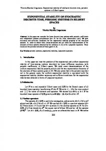
Therefore conditions (H4)–(H6) also hold. By Theorem 2, system (45) is exponentially stable in mean square. The EM scheme and the SSBE scheme to (45) are also MS stable by Theorems 5 and 7. Now, we can conclude that the EM method and the SSBE method to (45) are MS stable with ℎ = 0.125 from Figure 1. It verifies the validity of Theorems 5 and 7. The EM method is not stable, and the SSBE method is MS stable with ℎ = 0.1925
Abstract and Applied Analysis
9 1.4
1 0.9
1.2
0.8
1
0.7 E | x k |2
E | x k |2
0.6 0.5 0.4 0.3
0.6 0.4
0.2
0.2
0.1 0
0.8
0
5
10 tk
15
0
20
0
E|x1k |2
2
4
6
8
10 tk
12
14
16
18
20
E|x1k |2
E|x2k |2
E|x2k |2
(a)
(b)
Figure 1: MS stability of the numerical solutions to (45) with ℎ = 0.125; (a) EM, (b) SSBE. ×105 2
1
0.8
1.5
E | x k |2
E | x k |2
0.6 1
0.5
0
0.4
0.2
0
2
4
6
8 tk
10
12
14
16
0
5
0
10 tk
15
20
E|x1k |2
E|x1k |2
E|x2k |2
E|x2k |2
(a)
(b)
Figure 2: Instability of EM numerical solutions and MS stability of SSBE numerical solutions to (45) with ℎ = 0.1925; (a) EM, (b) SSBE.
from Figure 2, which shows that the stability of the SSBE method is more superior to EM. Figure 3 illustrates that the SSBE method is unstable with ℎ = 0.25.
6. Conclusions The model of stochastic neural network can be viewed as a special kind of stochastic differential equation; the solution is hard to be explicitly expressed. It not only has the
characteristics of the general stochastic differential equations but also has its own features; its stability is connected with the activation functions and the connection weight matrixes. So it is necessary to discuss the stability of stochastic neural network. Different from the previous works on exponential stability of stochastic neural networks, both Lyapunov function method and two numerical methods are used to study the stability of stochastic delay recurrent neural networks. Under the conditions which guarantee the stability of the analytical solution, the EM method and the SSBE method are
10
Abstract and Applied Analysis 4.5 4 3.5
E | x k |2
3 2.5 2 1.5 1 0.5 0
0
5
10 tk
15
20
E|x1k |2
E|x2k |2
Figure 3: Instability of SSBE numerical solutions of system (45) with ℎ = 0.25.
proved to be MS stable if the step size meets a certain limit. We can analyze other numerical methods for different types of stochastic delay neural networks in future.
Acknowledgments This work was supported by the National Natural Science Foundation of China (nos. 60904032, 61273126), the Natural Science Foundation of Guangdong Province (no. 10251064101000008), and the Fundamental Research Funds for the Central Universities (no. 2012ZM0059).
References [1] C. M. Marcus and R. M. Westervelt, “Stability of analog neural networks with delay,” Physical Review A, vol. 39, no. 1, pp. 347– 359, 1989. [2] J. Wu, Introduction to Neural Dynamics and Signal Transmission Delay, vol. 6, Walter de Gruyter, Berlin, Germany, 2001. [3] X. Li, L. Huang, and J. Wu, “Further results on the stability of delayed cellular neural networks,” IEEE Transactions on Circuits and Systems. I. Fundamental Theory and Applications, vol. 50, no. 9, pp. 1239–1242, 2003. [4] X. M. Li, L. H. Huang, and H. Zhu, “Global stability of cellular neural networks with constant and variable delays,” Nonlinear Analysis. Theory, Methods & Applications, vol. 53, no. 3-4, pp. 319–333, 2003. [5] S. Arik, “Stability analysis of delayed neural networks,” IEEE Transactions on Circuits and Systems. I. Fundamental Theory and Applications, vol. 47, no. 7, pp. 1089–1092, 2000. [6] S. Arik, “Global asymptotic stability analysis of bidirectional associative memory neural networks with time delays,” IEEE Transactions on Neural Networks, vol. 16, no. 3, pp. 580–586, 2005.
[7] T. Liao and F. Wang, “Global stability for cellular neural networks with time delay,” IEEE Transactions on Neural Networks, vol. 11, no. 6, pp. 1481–1484, 2000. [8] X. Liao, Q. Liu, and W. Zhang, “Delay-dependent asymptotic stability for neural networks with distributed delays,” Nonlinear Analysis. Real World Applications, vol. 7, no. 5, pp. 1178–1192, 2006. [9] S. Kuang, F. Deng, and X. Li, “Stability and hopf bifurcation of a BAM neural network with delayed self-feedback,” in Proceedings of the 7th International Symposium on Neural Networks, vol. 6063 of Lecture Notes in Computer Science, pp. 493–503, 2010. [10] O. Faydasicok and S. Arik, “Further analysis of global robust stability of neural networks with multiple time delays,” Journal of the Franklin Institute. Engineering and Applied Mathematics, vol. 349, no. 3, pp. 813–825, 2012. [11] S. Haykin, Neural Networks, Prentice-Hall, NJ, USA, 1994. [12] S. Blythe, X. Mao, and X. Liao, “Stability of stochastic delay neural networks,” Journal of the Franklin Institute, vol. 338, no. 4, pp. 481–495, 2001. [13] L. Wan and J. Sun, “Mean square exponential stability of stochastic delayed Hopfield neural networks,” Physics Letters A, vol. 343, no. 4, pp. 306–318, 2005. [14] Q. Zhou and L. Wan, “Exponential stability of stochastic delayed Hopfield neural networks,” Applied Mathematics and Computation, vol. 199, no. 1, pp. 84–89, 2008. [15] Y. Zhang, D. Yue, and E. Tian, “Robust delay-distributiondependent stability of discrete-time stochastic neural neural networks with time-varying delay,” Neurocomputing, vol. 72, no. 4, pp. 1265–1273, 2009. [16] Z. Wang, Y. Liu, M. Li, and X. Liu, “Stability analysis for stochastic Cohen-Grossberg neural networks with mixed time delay,” IEEE Transactions on Neural Networks, vol. 17, no. 3, pp. 814–820, 2006. [17] Y. Sun and J. Cao, “𝑝th moment exponential stability of stochastic recurrent neural networks with time-varying delays,” Nonlinear Analysis. Real World Applications, vol. 8, no. 4, pp. 1171–1185, 2007. [18] C. Huang, Y. He, and H. Wang, “Mean square exponential stability of stochastic recurrent neural networks with timevarying delays,” Computers & Mathematics with Applications, vol. 56, no. 7, pp. 1773–1778, 2008. [19] U. K¨uchler and E. Platen, “Strong discrete time approximation of stochastic differential equations with time delay,” Mathematics and Computers in Simulation, vol. 54, no. 1–3, pp. 189–250, 2000. [20] E. Buckwar, “Introduction to the numerical analysis of stochastic delay differential equations,” Journal of Computational and Applied Mathematics, vol. 125, no. 1-2, pp. 297–307, 2000. [21] D. J. Higham and P. E. Kloeden, “Convergence and stability of implicit methods for jump-diffusion systems,” International Journal of Numerical Analysis and Modeling, vol. 3, no. 2, pp. 125–140, 2006. [22] X. Mao and S. Sabanis, “Numerical solutions of stochastic differential delay equations under local Lipschitz condition,” Journal of Computational and Applied Mathematics, vol. 151, no. 1, pp. 215–227, 2003. [23] M. Liu, W. Cao, and Z. Fan, “Convergence and stability of the semi-implicit Euler method for a linear stochastic differential delay equation,” Journal of Computational and Applied Mathematics, vol. 170, no. 2, pp. 255–268, 2004.
Abstract and Applied Analysis [24] P. Hu and C. Huang, “Stability of stochastic 𝜃-methods for stochastic delay integro-differential equations,” International Journal of Computer Mathematics, vol. 88, no. 7, pp. 1417–1429, 2011. [25] A. Rathinasamy and K. Balachandran, “𝑇-stability of the splitstep 𝜃-methods for linear stochastic delay integro-differential equations,” Nonlinear Analysis. Hybrid Systems, vol. 5, no. 4, pp. 639–646, 2011. [26] H. Zhang, S. Gan, and L. Hu, “The split-step backward Euler method for linear stochastic delay differential equations,” Journal of Computational and Applied Mathematics, vol. 225, no. 2, pp. 558–568, 2009. [27] M. Song and H. Yu, “Numerical solutions of stochastic differential delay equations with Poisson random measure under the generalized Khasminskii-type conditions,” Abstract and Applied Analysis, vol. 2012, Article ID 127397, 24 pages, 2012. [28] Q. Li and S. Gan, “Stability of analytical and numerical solutions for nonlinear stochastic delay differential equations with jumps,” Abstract and Applied Analysis, vol. 2012, Article ID 831082, 13 pages, 2012. [29] X. Ding, K. Wu, and M. Liu, “Convergence and stability of the semi-implicit Euler method for linear stochastic delay integrodifferential equations,” International Journal of Computer Mathematics, vol. 83, no. 10, pp. 753–761, 2006. [30] R. Li, W. Pang, and P. Leung, “Exponential stability of numerical solutions to stochastic delay Hopfield neural networks,” Neurocomputing, vol. 73, no. 4–6, pp. 920–926, 2010. [31] F. Jiang and Y. Shen, “Stability in the numerical simulation of stochastic delayed Hopfield neural networks,” Neural Coputing and Applications, vol. 22, no. 7-8, pp. 1493–1498, 2013. [32] A. Rathinasamy, “The split-step 𝜃-methods for stochastic delay Hopfield neural networks,” Applied Mathematical Modelling, vol. 36, no. 8, pp. 3477–3485, 2012. [33] X. Mao, Stochastic Differential Equations and Applications, Horwood, Chichester, UK, 2nd edition, 2008.
11
Advances in
Operations Research Hindawi Publishing Corporation http://www.hindawi.com
Volume 2014
Advances in
Decision Sciences Hindawi Publishing Corporation http://www.hindawi.com
Volume 2014
Journal of
Applied Mathematics
Algebra
Hindawi Publishing Corporation http://www.hindawi.com
Hindawi Publishing Corporation http://www.hindawi.com
Volume 2014
Journal of
Probability and Statistics Volume 2014
The Scientific World Journal Hindawi Publishing Corporation http://www.hindawi.com
Hindawi Publishing Corporation http://www.hindawi.com
Volume 2014
International Journal of
Differential Equations Hindawi Publishing Corporation http://www.hindawi.com
Volume 2014
Volume 2014
Submit your manuscripts at http://www.hindawi.com International Journal of
Advances in
Combinatorics Hindawi Publishing Corporation http://www.hindawi.com
Mathematical Physics Hindawi Publishing Corporation http://www.hindawi.com
Volume 2014
Journal of
Complex Analysis Hindawi Publishing Corporation http://www.hindawi.com
Volume 2014
International Journal of Mathematics and Mathematical Sciences
Mathematical Problems in Engineering
Journal of
Mathematics Hindawi Publishing Corporation http://www.hindawi.com
Volume 2014
Hindawi Publishing Corporation http://www.hindawi.com
Volume 2014
Volume 2014
Hindawi Publishing Corporation http://www.hindawi.com
Volume 2014
Discrete Mathematics
Journal of
Volume 2014
Hindawi Publishing Corporation http://www.hindawi.com
Discrete Dynamics in Nature and Society
Journal of
Function Spaces Hindawi Publishing Corporation http://www.hindawi.com
Abstract and Applied Analysis
Volume 2014
Hindawi Publishing Corporation http://www.hindawi.com
Volume 2014
Hindawi Publishing Corporation http://www.hindawi.com
Volume 2014
International Journal of
Journal of
Stochastic Analysis
Optimization
Hindawi Publishing Corporation http://www.hindawi.com
Hindawi Publishing Corporation http://www.hindawi.com
Volume 2014
Volume 2014