Exposing the Probabilistic Causal Structure of Discrimination
Recommend Documents
Oct 5, 2015 - making, USA President Obama called for a 90-day review of big data ..... correlation information is called background knowledge, and is itself coded as an ..... ployment status and job status are defined in the second level.
Exposing Racial Discrimination - ResearchGate › publication › fulltext › Exposing-... › publication › fulltext › Exposing-...by N Krieger · 2011 · Cited by 77 · Related articlesNov 18, 2011 — Williams DR, Mohammed SA (2009) Discrimination and raci
Engineering Systems Department. Defence ... In this paper we propose PICI, probabilistic ICI, an extension of ..... Probabilistic Reasoning in Intelligent. Systems: ...
Jan 26, 2016 - Joonwoo Bae 1,*, Dai-Gyoung Kim 1 and Leong-Chuan Kwek 2,3,4,5. 1 ... Keywords: optimal state discrimination; generalized probabilistic theories; ..... Exploiting the convex geometry, see Figure 2, the polytope P({1/4, wx}3.
Nov 18, 2011 - Black & White Community Health Center Members ... United States of America, 2 Haas School of Business, ... Association Test (IAT) for racial discrimination, first developed and used in two recent published studies, and measured .... st
library, called Causal Explorer, that implements a suit of global, local and partial CPN induction ... Networks (BNs) [3] in which edges between any two variables in the graph denote direct causal relationships between .... the provided API. 4.2.
May 8, 2006 - A large data set has been generated using three biological replicates of each isolate and three ... Ordination plots generated using the PC-DFA are presented .... The recovery of the Enterococcus spp. from the other bacteria is ...
Nov 24, 2013 - Job Services Australia (JSA) which was established to assist people in .... barriers included: distance to jobs or lack of transport; too many ...
ÏBCâ/CÎ A â nâ1â/BnD/4Î A. (41). + âi. (ÏAiB¯kCN â ÏBC¯kAiN + RCAi4B)Î A1.. ËC..Am . Also, for a scalar function f,. â/N â/Af â â/Aâ/N f = â. 3. 2. kAN D4f ...
areas, though civilian aircraft may also appear in these areas accidentally. ... E. Waltz and J. Llinas, Multisensor Data Fusion, Artech House, Boston, 1990. 13.
This originated a growing interest in the field of Probabilistic Inductive Logic Programming, which ... In this paper we present the algorithm SLIPCASE for âStructure LearnIng of .... All experiments were performed on Linux machines with an.
Dec 7, 2015 - 1)Institute of Cosmology and Gravitation, University of Portsmouth, ... three-dimensional matter field and its formation history. To allow feasible ...
teleseismic Pwaves. MERMAID RAFOS float (constructed by Teledyne Web Research) equipped with a hydrophone to detect acoustic signals generated by.
7604. 3256. Table . The gender-income contingency table of the test-set. This changes .... several analysis techniques like ROC (receiver operator curve) analysis (Lachiche ... attribute from the data-set used to train the Naive Bayes classifier.
Feb 4, 2009 - arXiv:0808.3844v2 [quant-ph] 4 Feb 2009. Optimal State Discrimination in General Probabilistic Theories. Gen Kimura [a],â Takayuki Miyadera ...
David A. Lagnado ([email protected]). Department ... action from observation (Pearl, 2000). .... Pearl (2000) achieves this through the introduction of.
May 21, 2014 - demonstrate a causal link between the L-OTC and mirror-image discrimination in literate ... occipitotemporal cortex, visual word-form area.
Apr 30, 2009 - By a theorem of David Malament and others [13, 14], we know that the ...... [28] Brightwell G 1993 Surveys in Combinatorics (London Math. Soc.
by a National Institute of Mental Health Individual Postdoctoral Fel- lowship to Laura ..... of norms (i.e., "presuppositions about what a class of persons generally does to ...... faulty rail, and the weight of the cars may all have been necessary f
object that enters into an affordance model on the right, with physical structure as the overlapping element. We have ad
May 16, 2007 - Indeed if at i sites one collects the areas Ai and must enforce the con- straint ...... See color version
ly, knowledge of the causal relations that link the features of categoriesâsupports the ability to infer the presence of unobserved features. Our experiments were ...
how well the name âmopâ applied to the object in a scenario, they would retrieve the ideal ..... good category membe
Similarly, if only agent goal is compromised, a slight drop in ratings should result, ..... nent was presented in a text
Exposing the Probabilistic Causal Structure of Discrimination
Oct 5, 2015 - on random walks on top of the SBCN, addressing differ- ..... 2. it proposes a holistic approach able to deal with differ- ..... a commodity laptop.
Exposing the Probabilistic Causal Structure of Discrimination Francesco Bonchi1,2
arXiv:1510.00552v3 [cs.DB] 8 Mar 2017
1
Sara Hajian2
Bud Mishra3
2
3
Algorithmic Data Analytics Lab ISI Foundation, Turin, Italy
ABSTRACT Discrimination discovery from data is an important task aiming at identifying patterns of illegal and unethical discriminatory activities against protected-by-law groups, e.g., ethnic minorities. While any legally-valid proof of discrimination requires evidence of causality, the state-of-theart methods are essentially correlation-based, albeit, as it is well known, correlation does not imply causation. In this paper we take a principled causal approach to the data mining problem of discrimination detection in databases. Following Suppes’ probabilistic causation theory, we define a method to extract, from a dataset of historical decision records, the causal structures existing among the attributes in the data. The result is a type of constrained Bayesian network, which we dub Suppes-Bayes Causal Network (SBCN). Next, we develop a toolkit of methods based on random walks on top of the SBCN, addressing different anti-discrimination legal concepts, such as direct and indirect discrimination, group and individual discrimination, genuine requirement, and favoritism. Our experiments on real-world datasets confirm the inferential power of our approach in all these different tasks.
1.
INTRODUCTION
The importance of discrimination discovery. At the beginning of 2014, as an answer to the growing concerns about the role played by data mining algorithms in decisionmaking, USA President Obama called for a 90-day review of big data collecting and analysing practices. The resulting report1 concluded that “big data technologies can cause societal harms beyond damages to privacy”. In particular, it expressed concerns about the possibility that decisions informed by big data could have discriminatory effects, even in the absence of discriminatory intent, further imposing less favorable treatment to already disadvantaged groups. 1 http://www.whitehouse.gov/sites/default/files/ docs/big_data_privacy_report_may_1_2014.pdf
Permission to make digital or hard copies of all or part of this work for personal or classroom use is granted without fee provided that copies are not made or distributed for profit or commercial advantage and that copies bear this notice and the full citation on the first page. To copy otherwise, to republish, to post on servers or to redistribute to lists, requires prior specific permission and/or a fee. Copyright 20XX ACM X-XXXXX-XX-X/XX/XX ...$10.00.
Discrimination refers to an unjustified distinction of individuals based on their membership, or perceived membership, in a certain group or category. Human rights laws prohibit discrimination on several grounds, such as gender, age, marital status, sexual orientation, race, religion or belief, membership in a national minority, disability or illness. Anti-discrimination authorities (such as equality enforcement bodies, regulation boards, consumer advisory councils) monitor, provide advice, and report on discrimination compliances based on investigations and inquiries. A fundamental role in this context is played by discrimination discovery in databases, i.e., the data mining problem of unveiling discriminatory practices by analyzing a dataset of historical decision records. Discrimination is causal. According to current legislation, discrimination occurs when a group is treated “less favorably” [1] than others, or when “a higher proportion of people not in the group is able to comply” with a qualifying criterion [2]. Although these definitions do not directly imply causation, as stated in [3] all discrimination claims require plaintiffs to demonstrate a causal connection between the challenged outcome and a protected status characteristic. In other words, in order to prove discrimination, authorities must answer the counterfactual question: what would have happened to a member of a specific group (e.g., nonwhite), if he or she had been part of another group (e.g., white)? “The Sneetches”, the popular satiric tale2 against discrimination published in 1961 by Dr. Seuss, describes a society of yellow creatures divided in two races: the ones with a green star on their bellies, and the ones without. The StarBelly Sneetches have some privileges that are instead denied to Plain-Belly Sneetches. There are, however, Star-On and Star-Off machines that can make a Plain-Belly into a StarBelly, and viceversa. Thanks to these machines, the causal relationship between race and privileges can be clearly measured, because stars can be placed on or removed from any belly, and multiple outcomes can be observed for an individual. Therefore, we could readily answer the counterfactual question, saying with certainty what would have happened to a Plain-Belly Sneetch had he or she been a Star-Belly Sneetch. In the real world however, proving discrimination episodes is much harder, as we cannot manipulate race, gender, or sexual orientation of an individual. This highlights the need to assess discrimination as a causal inference problem [4] 2 http://en.wikipedia.org/wiki/The_Sneetches_and_ Other_Stories
from a database of past decisions, where causality can be inferred probabilistically. Unfortunately, the state of the art of data mining methods for discrimination discovery in databases does not properly address the causal question, as it is mainly based on correlation-based methods (surveyed in Section 2). Correlation is not causation. It is well known that correlation between two variables does not necessarily imply that one causes the other. Consider a unique cause X of two effects, Y and Z: if we do not take into account X, we might derive wrong conclusions because of the observable correlation between Y and Z. In this situation, X is said to act as a confounding factor for the relationship between Y and Z. Variants of the complex relation just discussed can arise even if, in the example, X is not the actual cause of either Y or Z, but it is only correlated to them, for instance, because of how the data were collected. Consider for instance a credit dataset where there exists high correlation between a variable representing low income and another variable representing loan denial and let us assume that this is due to an actual legitimate causal relationship in the sense that, legitimately, a loan is denied if the applicant has low income. Let us now assume that we also observe high correlation between low income and being female, which, for instance, can be due to the fact that the women represented in the specific dataset in analysis, tend to be underpaid. Given these settings, in the data we would also observe high correlation between the variable gender being female and the variable representing loan denial, due to the fact that we do not account for the presence of the variable low income. Following common terminologies, we will say that such situations are due to spurious correlations. However, the picture is even more complicated: it could be the case, in fact, that being female is the actual cause of the low income and, hence, be the indirect cause of loan denial through low income. This would represent a causal relationship between the gender and the loan denial, that we would like to detect as discrimination. Disentangling these two different cases, i.e., female is only correlated to low income in a spurious way, or being female is the actual cause of low income, is at the same time important and challenging. This highlights the need for a principled causal approach to discrimination detection. Another typical pitfall of correlation-based reasoning is expressed by what is known as Simpson’s paradox3 according to which, correlations observed in different groups might disappear when these heterogeneous groups are aggregated, leading to false positives cases of discrimination discovery. One of the most famous false-positive examples due to Simpson’s paradox occurred when in 1973 the University of California, Berkeley was sued for discrimination against women who had applied for admission to graduate schools. In fact, by looking at the admissions of 1973, it first appeared that men applying were significantly more likely to be admitted than women. But later, by examining the individual departments carefully, it was discovered that none of them was significantly discriminating against women. On the contrary, most departments had exercised a small bias in favor of women. The apparent discrimination was due to the fact that women tended to apply to departments with lower 3
http://en.wikipedia.org/wiki/Simpson’s_paradox
rates of admission, while men tended to apply to departments with higher rates [5]. Later in Section 5.5 we will use the dataset from this episode to highlight the differences between correlation-based and causation-based methods. Spurious correlations can also lead to false negatives (i.e., discrimination existing but not being detected) as is commonly seen in “reverse-discrimination”. The typical case is when authorities take affirmative actions, e.g., with compensatory quota systems, in order to protect a minority group from a potential discrimination. Such actions, while trying to erase the supposed discrimination (i.e., the spurious correlation), fail to address the real underlying causes for discrimination, potentially ending up denying individual members of a privileged group from access to their rightful shares of social goods. In the early 70’s, a case involving the University of California at Davis Medical School highlighted one such incident as the school’s admissions program reserved 16 of the 100 places in its entering class for “disadvantaged” applicants, thus unintentionally reducing the chances of admission for a qualified applicant.4 These are just few typical examples of the pitfalls of correlation-based reasoning in the discovery of discrimination. Later in Section 5.5 we show concrete examples from real-world datasets where correlation-based methods to discrimination discovery are not satisfactory. Our proposal and contributions. In this paper we take a principled causal approach to the data mining problem of discrimination detection in databases. Following Suppes’ probabilistic causation theory [6, 7] we define a method to extract, from a dataset of historical decision records, the causal structures existing among the attributes in the data. In particular, we define the Suppes-Bayes Causal Network (SBCN), i.e., a directed acyclic graph (dag) where we have a node representing a Bernulli variable of the type hattribute = valuei for each pair attribute-value present in the database. In this dag an arc (A, B) represents the existence of a causal relation between A and B (i.e., A causes B). Moreover, each arc is labeled with a score, representing the strength of the causal relation. Our SBCN is a constrained Bayesian network reconstructed by means of maximum likelihood estimation (MLE) from the given database, where we force the conditional probability distributions induced by the reconstructed graph to obey Suppes’ constraints: i.e., temporal priority and probability rising. Imposing Suppes’ temporal priority and probability raising we obtain what we call the prima facie causes graph [7], which might still contain spurious causes (false positives). In order to remove these spurious case we add a bias term to the likelihood score, favoring sparser causal networks: in practice we sparsify the prima facie causes graph by extracting a minimal set of edges which best explain the data. This regularization is done by means of the Bayesian Information Criterion (BIC) [8]. The obtained SBCN provides a clear summary, amenable to visualization, of the probabilistic causal structures found in the data. Such structures can be used to reason about different types of discrimination. In particular, we show how using several random-walk-based methods, where the next step in the walk is chosen proportionally to the edge weights, we can address different anti-discrimination legal concepts. 4 http://en.wikipedia.org/wiki/Regents_of_the_ University_of_California_v._Bakke
Our experiments show that the measures of discrimination produced by our methods are very strong, almost binary, signals: our measures are very clearly separating the discrimination and the non-discrimination cases. To the best of our knowledge this is the first proposal of discrimination detection in databases grounded in probabilistic causal theory. Roadmap. The rest of the paper is organized as follows. Section 2 discusses the state of the art in discrimination detection in databases. In Section 3 we formally introduce the SBCN and we present the method for extracting such causal network from the input dataset. Once extracted our SBCN, in Section 4 we show how to exploit it for different concepts of discrimination detection, by means of randomwalk methods. Finally Section 5 presents our experimental assessment and comparison with correlation-based methods on two real-world datasets.
2.
as a tool for discrimination discovery. Bayesian networks consider the dependence between all the attributes and use these dependencies in estimating the joint probability distribution without any strong assumption, since a Bayesian network graphically represents a factorization of the joint distribution in terms of conditional probabilities encoded in the edges. Although Bayesian networks are often used to represent causal relationships, this needs not be the case, in fact a directed edge from two nodes of the network does not imply any causal relation between them. As an example, let us observe that the two graphs A → B → C and C → B → A impose exactly the same conditional independence requirements and, hence, any Bayesian network would not be able to disentangle the direction of any causal relationship among these events. Our work departs from this literature as: 1. it is grounded in probabilistic causal theory instead of being based on correlation;
RELATED WORK
Discrimination analysis is a multi-disciplinary problem, involving sociological causes, legal reasoning, economic models, statistical techniques [9, 10]. Some authors [11, 12] study how to prevent data mining from becoming itself a source of discrimination. In this paper instead we focus on the data mining problem of detecting discrimination in a dataset of historical decision records, and in the rest of this section we present the most related literature. Pedreschi et al. [13, 14, 15] propose a technique based on extracting classification rules (inductive part) and ranking the rules according to some legally grounded measures of discrimination (deductive part). The result is a (possibly large) set of classification rules, providing local and overlapping niches of possible discrimination. This model only deals with group discrimination. Luong et al. [16] exploit the idea of situation-testing [17] to detect individual discrimination. For each member of the protected group with a negative decision outcome, testers with similar characteristics (k-nearest neighbors) are considered. If there are significantly different decision outcomes between the testers of the protected group and the testers of the unprotected group, the negative decision can be ascribed to discrimination. Zliobaite et al. [18] focus on the concept of genuine requirement to detect that part of discrimination which may be explained by other, legally grounded, attributes. In [19] Dwork et al. address the problem of fair classification that achieves both group fairness, i.e., the proportion of members in a protected group receiving positive classification is identical to the proportion in the population as a whole, and individual fairness, i.e., similar individuals should be treated similarly. The above approaches assume that the dataset under analysis contains attributes that denote protected groups (i.e., direct discrimination). This may not be the case when such attributes are not available, or not even collectable at a micro-data level as in the case of the loan applicant’s race. In these cases we talk about indirect discrimination discovery. Ruggieri et al. [20, 21] adopt a form of rule inference to cope with the indirect discovery of discrimination. The correlation information is called background knowledge, and is itself coded as an association rule. Mancuhan and Clifton [22] propose Bayesian networks
2. it proposes a holistic approach able to deal with different types of discrimination in a single unifying framework, while the methods in the state of the art usually deal with one and only one specific type of discrimination; 3. it is the first work to adopt graph theory and social network analysis concepts, such as random-walk-based centrality measures and community detection, for discrimination detection; Our proposal has also lower computational cost than methods such as [13, 14, 15] which require to compute a potentially exponential number of association/classification rules.
3.
SUPPES-BAYES CAUSAL NETWORK
In order to study discrimination as a causal inference problem, we exploit the criteria defined in the theories of probabilistic causation [6]. In particular, we follow [7], where Suppes proposed the notion of prima facie causation that is at the core of probabilistic causation. Suppes’ definition is based on two pillars: (i) any cause must happen before its effect (temporal priority) and (ii) it must raise the probability of observing the effect (probability raising). Definition 1 (Probabilistic causation [7]). For any two events h and e, occurring respectively at times th and te , under the mild assumptions that 0 < P(h), P(e) < 1, the event h is called a prima facie cause of the event e if it occurs before the effect and the cause raises the probability of the effect, i.e. th < te and P(e | h) > P(e | ¬h) . In the rest of this section we introduce our method to construct, from a given relational table D, a type of causal Bayesian network constrained to satisfy the conditions dictated by Suppes’ theory, which we dub Suppes-Bayes Causal Network (SBCN). In the literature many algorithms exist to carry out structural learning of general Bayesian networks and they usually fall into two families [23]. The first family, constraint based learning, explicitly tests for pairwise independence of variables conditioned on the power set of the rest of the variables in the network. These algorithms exploit structural conditions defined in various approaches to causality [6, 24, 25]. The second family, score based learning, constructs
a network which maximizes the likelihood of the observed data with some regularization constraints to avoid overfitting. Several hybrid approaches have also been recently proposed [26, 27, 28]. Our framework can be considered a hybrid approach exploiting constrained maximum likelihood estimation (MLE) as follows: (i) we first define all the possible causal relationship among the variables in D by considering only the oriented edges between events that are consistent with Suppes’ notion of probabilistic causation and, subsequently, (ii) we perform the reconstruction of the SBCN by a score-based approach (using BIC), which considers only the valid edges. We next present in details the whole learning process.
3.1
Suppes’ constraints
We start with an input relational table D defined over a set A of h categorical attributes and s samples. In case continuous numerical attributes exists in D, we assume they have been discretized to become categorical. From D, we derive D0 , an m × s binary matrix representing m Bernoulli variables of the type hattribute = valuei, where an entry is 1 if we have an observation for the specific variable and 0 otherwise. Temporal priority. The first constraint, temporal priority, cannot be simply checked in the data as we have no timing information for the events. In particular, in our context the events for which we want to reason about temporal priority are the Bernoulli variables hattribute = valuei. The idea here is that, e.g., income = low cannot be a cause of gender = f emale, because the time when the gender of an individual is determined is antecedent to that of when the income is determined. This intuition is implemented by simply letting the data analyst provide as input to our framework a partial temporal order r : A → N for the h attributes, which is then inherited from the m Bernoulli variables 5 . Based on the input dataset D and the partial order r we produce the first graph G = (V, E) where we have a node for each of the Bernoulli variables, so |V | = m, and we have an arc (u, v) ∈ E whenever r(u) ≤ r(v). This way we will immediately rule out causal relations that do not satisfy the temporal priority constraint. Probability raising. Given the graph G = (V, E) built as described above the next step requires to prune the arcs which do not satisfy the second constraint, probability raising, thus building G0 = (V, E 0 ), where E 0 ⊆ E. In particular we remove from E each arc (u, v) such that P(v | u) ≤ P(v | ¬u). The graph G0 so obtained is called prima facie graph. We recall that the probability raising condition is equivalent to constraining for positive statistical dependence [27]: in the prima facie graph we model all and only the positive correlated relations among the nodes already partially ordered by temporal priority, consistently with Suppes’ characterization of causality in terms of relevance. 5 Note that our learning technique requires the input order r to be correct and complete in order to guarantee its convergence. Nevertheless, if this is not the case, it is still capable of providing valuable insights about the underlying causal model, although with the possibility of false positive or false negative causal claims.
3.2
Network simplification
Suppes’ conditions are necessary but not sufficient to evaluate causation [28]: especially when the sample size is small, the model may have false positives (spurious causes), even after constraining for Suppes’ temporal priority and probability raising criteria (which aim at removing false negatives). Consequently, although we expect all the statistically relevant causal relations to be modelled in G0 , we also expect some spurious ones in it. In our proposal, in place of other structural conditions used in various approaches to causality, (see e.g., [6, 24, 25]), we perform a network simplification (i.e., we sparsify the network by removing arcs) with a score based approach, specifically by relying on the Bayesian Information Criterion (BIC) as the regularized likelihood score [8]. We consider as inputs for this score the graph G0 and the dataset D0 . Given these, we select the set of arcs E ∗ ⊆ E 0 that maximizes the score: scoreBIC (D0 , G0 ) = LL(D0 |G0 ) −
log s dim(G0 ). 2
In the equation, G0 denotes the graph, D0 denotes the data, s denotes the number of samples, and dim(G0 ) denotes the number of parameters in G0 . Thus, the regularization term −dim(G0 ) favors graphs with fewer arcs. The coefficient log s/2 weighs the regularization term, such that the higher the weight, the more sparsity will be favored over “explaining” the data through maximum likelihood. Note that the likelihood is implicitly weighted by the number of data points, since each point contributes to the score. Assume that there is one true (but unknown) probability distribution that generates the observed data, which is, eventually, uniformly randomly corrupted by false positives and negatives rates (in [0, 1)). Let us call correct model, the statistical model which best approximate this distribution. The use of BIC on G0 results in removing the false positives and, asymptotically (as the sample size increases), converges to the correct model. In particular, BIC is attempting to select the candidate model corresponding to the highest Bayesian Posterior probability, which can be proved to be equivalent to the presented score and its log(s) penalization factor. We denote with G∗ = (V, E ∗ ) the graph that we obtain after this step. We note that, as for general Bayesian network, G∗ is a dag by construction.
3.3
Confidence score
Using the reconstructed SBCN, we can represent the probabilistic relationships between any set of events (nodes). As an example, suppose to consider the nodes representing respectively income = low and gender = f emale being the only two direct causes (i.e., with arcs toward) of loan = denial. Given SBCN, we can estimate the conditional probabilities for each node in the graph, i.e., probability of loan = denial given income = low AN D gender = f emale in the example, by computing the conditional probability of only the pair of nodes directly connected by an arc. For an overview of state-of-the-art methods for doing this, see [23]. However, we expect to be mostly dealing with full data, i.e., for every directly connected node in the SBCN, we expect to have several observations of any possible combination attribute = value. For this reason, we can simply estimate the node probabilities by counting the observations
native_country_India 0.213 sex_Male 0.11 0.456
age_old 0.39
0.011 0.06 0.157
marital_status_Married_civ_spouse 0.006
0.069
0.052
0.038
education_Assoc_voc 0.035
0.382
0.028
0.328
0.141
workclass_Self_emp_not_inc
0.159
0.06
positive_dec
relationship_Husband
0.178
0.066
occupation_Exec_managerial
0.151
0.272 0.076
0.492
0.509
0.066
occupation_Craft_repair
workclass_Local_gov
workclass_State_gov
0.132
0.371 0.015
0.019
education_Prof_school 0.122
workclass_Self_emp_inc
0.088
0.129
0.018
education_Masters 0.153
0.208 0.059
0.88 0.085
0.267
0.604
native_country_Cuba
0.026
education_Bachelors
0.019
0.002
0.012 0.35
0.656
0.043 0.611
occupation_Prof_specialty 0.036
education_Doctorate
0.172 0.001 workclass_Never_worked
0.071
occupation_Protective_serv
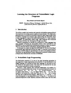
Figure 1: One portion of the SBCN extracted from the Adult dataset. This subgraph corresponds to the C2 community reported later in Table 3 (Section 5) extracted by a community detection algorithm. in the data. Moreover, we will exploit such conditional probabilities to define the confidence score of each arc in terms of their causal relationship. In particular, for each arc (v, u) ∈ E ∗ involving the causal relationship between two nodes u, v ∈ V , we define a confidence score W (v, u) = P(u | v) − P(u | ¬v), which, intuitively, aims at estimating the observations where the cause v is followed by its effect u, that is P(u | v), and the ones where this is not observed, i.e., P(u | ¬v), because of imperfect causal regularities. We also note that, by the constraints discussed above, we require P(u | v) P(u | ¬v) and, for this reason, each weight is positive and no larger than 1, i.e., W : E ∗ → (0, 1]. Combining all of the concepts discussed above, we conclude with the following definition. Definition 2 (Suppes-Bayes Causal Network). Given an input dataset D0 of m Bernoulli variables and s samples, and given a partial order r of the variables, the Suppes-Bayes Causal Network SBCN = (V, E ∗ , W ) subsumed by D0 is a weighted dag such that the following requirements hold: • [Suppes’ constraints] for each arc (v, u) ∈ E ∗ involving the causal relationship between nodes u, v ∈ V , under the mild assumptions that 0 < P(u), P(v) < 1: r(v) ≤ r(u)
and
P(u | v) > P(u | ¬v) .
0
• [Simplification] let E be the set of arcs satisfying the Suppes’ constraints as before; among all the subsets of E 0 , the set of arcs E ∗ is the one whose corresponding graph maximizes BIC: E∗ =
arg max
(LL(D0 |G) −
E⊆E 0 ,G=(V,E)
log s dim(G)) . 2
• [Score] W (v, u) = P(u | v) − P(u | ¬v), ∀(v, u) ∈ E ∗
An example of a portion of a SBCN extracted from a realworld dataset is reported in Figure 1. Algorithm 1 summarizes the learning approach adopted for the inference of the SBCN . Given D0 an input dataset over m Bernoulli variables and s samples, and r a partial order of the variables, Suppes’ constraints are verified (Lines 4-9) to construct a dag as described in Section 3.1. The likelihood fit is performed by hill climbing (Lines 1221), an iterative optimization technique that starts with an arbitrary solution to a problem (in our case an empty graph) and then attempts to find a better solution by incrementally visiting the neighbourhood of the current one. If the new candidate solution is better than the previous one it is considered in place of it. The procedure is repeated until the stopping criterion is matched. The !StoppingCriterion occurs (Line 12) in two situations: (i) the procedure stops when we have performed a large enough number of iterations or, (ii) it stops when none of the solutions in Gneighbors is better than the current Gf it . Note that Gneighbors denotes all the solutions that are derivable from Gf it by removing or adding at most one edge.
Time and space complexity. The computation of the valid dag according to Suppes’ constraints (Lines 4-10) requires a pairwise calculation among the m Bernoulli variables. After that, the likelihood fit by hill climbing (Lines 11-21) is performed. Being an heuristic, the computational cost of hill climbing depends on the sopping criterion. However, constraining by Suppes’ criteria tends to regularize the problem leading on average to a quick convergence to a good solution. The time complexity of Algorithm 1 is O(sm) and the space required is O(m2 ), where m however is usually not too large, being the number of attribute-value pairs, and not the number of examples.
Algorithm 1 Learning the SBCN 1: Inputs: D0 an input dataset of m Bernoulli variables and s samples, and r a partial order of the variables 2: Output: SBCN (V, E ∗ , W ) as in Definition 2 3: [Suppes’ constraints] 4: for all pairs (v, u) among the m Bernoulli variables do 5: if r(v) ≤ r(u) and P(u | v) > P(u | ¬v) then 6: add the arc (v, u) to SBCN . 7: end if 8: end for 9: [Likelihood fit by hill climbing] 10: Consider G(V, E ∗ , W )f it = ∅. 11: while !StoppingCriterion() do 12: Let G(V, E ∗ , W )neighbors be the neighbor solutions of G(V, E ∗ , W )f it . 13: Remove from G(V, E ∗ , W )neighbors any solution whose arcs are not included in SBCN . 14: Consider a random solution Gcurrent in G(V, E ∗ , W )neighbors . 15: if scoreBIC (D0 , Gcurrent ) > scoreBIC (D0 , Gf it ) then 16: Gf it = Gcurrent . 17: ∀ arc (v, u) of Gf it , W (v, u) = P(u | v)−P(u | ¬v). 18: end if 19: end while 20: SBCN = Gf it . 21: return SBCN .
3.4
Expressivity of a SBCN
We conclude this Section with a discussion on the causal relations that we model by a SBCN . Let us assume that there is one true (but unknown) probability distribution that generates the observed data whose structure can be modelled by a dag. Furthermore, let us consider the causal structure of such a dag and let us also assume each node with more then one cause to have conjunctive parents: any observation of the child node is preceded by the occurrence of all its parents. As before we call correct model, the statistical model which best approximate the distribution. On these settings, we can prove the following theorem. Theorem 1. Let the sample size s → ∞, the provided partial temporal order r be correct and complete and the data be uniformly randomly corrupted by false positives and negatives rates (in [0, 1)), then the SBCN inferred from the data is the correct model. Proof. [Sketch] Let us first consider the case where the observed data have no noise. On such an input, we observe that the prima facie graph has no false negatives: in fact ∀[c → e] modelling a genuine causal relation, P(e ∧ c) = P(e), thus the probability raising constraint is satisfied, so it is the temporal priority given that we assumed r to be correct and complete. Furthermore, it is know that the likelihood fit performed by BIC converges to a class of structures equivalent in terms of likelihood among which there is the correct model: all these topologies are the same unless the directionality of some edges. But, since we started with the prima facie graph which is already ordered by temporal priority, we can conclude that in this case the SBCN coincides with the correct model.
To extend the proof to the case of data uniformly randomly corrupted by false positives and negatives rates (in [0, 1)), we note that the marginal and joint probabilities change monotonically as a consequence of the assumption that the noise is uniform. Thus, all inequalities used in the preceding proof still hold, which concludes the proof. In the more general case of causal topologies where any cause of a common effect is independent from any other cause (i.e., we relax the assumption of conjunctive parents), the SBCN is not guaranteed to converge to the correct model but it coincides with a subset of it modeling all the edges representing statistically relevant causal relations (i.e., where the probability raising condition is verified).
4.
DISCRIMINATION RANDOM WALKS
DISCOVERY
BY
In this section we propose several random-walk-based methods over the reconstructed SBCN, to deal with different discrimination-detection tasks.
4.1
Group discrimination and favoritism
The basic problem in the analysis of direct discrimination is precisely to quantify the degree of discrimination suffered by a given protected group (e.g., an ethnic group) with respect to a decision (e.g., loan denial). In contrast to discrimination, favoritism refers to the case of an individual treated better than others for reasons not related to individual merit or business necessity: for instance, favoritism in the workplace might result in a person being promoted faster than others unfairly. In the following we denote favoritism as positive discrimination in contrast with negative discrimination. Given an SBCN we define a measure of group discrimination (either negative or positive) for each node v ∈ V . Recall that each node represents a pair hattribute = valuei, so it is essentially what we refer to as a group, e.g., hgender = f emalei. Our task is to assign a score of discrimination ds− : V → [0, 1] to each node, so that the closer ds− (v) is to 1 the more discriminated is the group represented by v. We compute this score by means of a number n of random walks that start from v and reaches either the node representing the positive decision or the one representing the negative decision. In these random walks the next step is chosen proportionally to the weights of the out-going arcs. Suppose a random walk has reached a node u, and let degout (u) denote the set of outgoing arcs from u. Then the arc (u, z) is chosen with probability p(u, z) = P
W (u, z) . e∈degout (u) W (e)
When a random walk ends in a node with no outgoing arc before reaching either the negative or the positive decision, it is restarted from the source node v. Definition 3 (Group discrimination score). Given an SBCN = (V, E ∗ , W ), let δ − ∈ V and δ + ∈ V denote the nodes indicating the negative and positive decision, respectively. Given a node v ∈ V , and a number n ∈ N of random walks to be performed, we denote as rwv→δ− the number of random walks started at node v that reach δ − earlier than δ + . The discrimination score for
the group corresponding to node v is then defined as ds− (v) =
rwv→δ− . n
This implicitly also defines a score of positive discrimination (or favoritism): ds+ (v) = 1 − ds− (v). Taking advantage of the SBCN we also propose two additional measures capturing how far a node representing a group is from the positive and negative decision respectively. This is done by computing the average number of steps that the random walks take to reach the two decisions: we denote these scores as as− (v) and as+ (v).
4.2
Indirect discrimination
The European Union Legislation [2] provides a broad definition of indirect discrimination as occurring “where an apparently neutral provision, criterion or practice would put persons of a racial or ethnic origin at a particular disadvantage compared with other persons”. In other words, the actual result of the apparently neutral provision is the same as an explicitly discriminatory one. A typical legal case study of indirect discrimination is concerned with redlining: e.g., denying a loan because of ZIP code, which in some areas is an attribute highly correlated to race. Therefore, even if the attribute race cannot be required at loan-application time (thus would not be present in the data), still race discrimination is perpetrated. Indirect discrimination discovery refers to the data mining task of discovering the attributes values that can act as a proxy to the protected groups and lead to discriminatory decisions indirectly [13, 14, 11]. In our setting, indirect discrimination can be detected by applying the same method described in Section 4.1.
4.3
4.4
Individual discrimination requires to measure the amount of discrimination for a specific individual, i.e., an entire record in the database. Similarly, subgroup discrimination refers to discrimination against a subgroup described by a combination of multiple protected and non-protected attributes: personal data, demographics, social, economic and cultural indicators, etc. For example, consider the case of gender discrimination in credit approval: although an analyst may observe that no discrimination occurs in general, it may turn out that older women obtain car loans only rarely. Both problems can be handled by generalizing the technique introduced in Section 4.1 to deal with a set of starting nodes, instead of only one. Given an SBCN = (V, E ∗ , W ) let v1 , . . . , vn be the nodes of interest. In order to define a discrimination score for v1 , . . . , vn , we perform a personalized PageRank [32] computation with respect to v1 , . . . , vn . In personalized PageRank, the probability of jumping to a node when abandoning the random walk is not uniform, but it is given by a vector of probabilities for each node. In our case the vector will have the value n1 for each of the nodes v1 , ..., vn ∈ V and zero for all the others. The output of personalized PageRank is a score ppr(u|v1 , ..., vn ) of proximity/relevance to {v1 , ..., vn } for each other node u in the network. In particular, we are interested in the score of the nodes representing the negative and positive decision: i.e., ppr(δ − |v1 , ..., vn ) and ppr(δ + |v1 , ..., vn ) respectively. Definition 4 (Generalized discrimination score). Given an SBCN = (V, E ∗ , W ), let δ − ∈ V and δ + ∈ V denote the nodes indicating the negative and positive decision, respectively. Given a set of nodes v1 , ..., vn ∈ V , we define the generalized (negative) discrimination score for the subgroup or the individual represented by {v1 , ..., vn } as
Genuine requirement
The legal concept of genuine requirement refers to detecting that part of the discrimination which may be explained by other, legally-grounded, attributes; e.g., denying credit to women may be explainable by the fact that most of them have low salary or delay in returning previous credits. A typical example in the literature is the one of the “genuine occupational requirement”, also called “business necessity” in [29, 30]. In the state of the art of data mining methods for discrimination discovery, it is also known as explainable discrimination [31] and conditional discrimination [18]. The task here is to evaluate to which extent the discrimination apparent for a group is “explainable” on a legal ground. Let v ∈ V be the node representing the group which is suspected of being discriminated, and ul ∈ V be a node whose causal relation with a negative or positive decision is legally grounded. As before, δ − and δ + denote the negative and positive decision, respectively. Following the same random-walk process described in Section 4.1, we define the fraction of explainable discrimination for the group v: f ed− (v) =
rwv→ul →δ− , rwv→δ−
i.e., the fraction of random walks passing trough ul among the ones started in v and reaching δ − earlier than δ + . Similarly we define f ed+ (v), i.e., the fraction of explainable positive discrimination.
This implicitly also defines a generalized score of positive discrimination: gds+ (v1 , ..., vn ) = 1 − gds− (v1 , ..., vn ).
5.
EXPERIMENTAL EVALUATION
This section reports the experimental evaluation of our approach on four datasets, Adult, German credit and census-income from the UCI Repository of Machine Learning Databases6 , and Berkeley Admissions Data from [34]. These are well-known real-life datasets typically used in discrimination-detection literature. Adult: consists of 48,842 tuples and 10 attributes, where each tuple correspond to an individual and it is described by personal attributes such as age, race, sex, relationship, education, employment, etc. Following the literature, in order to define the decision attribute we use the income levels, ≤50K (negative decision) or >50K (positive decision). We use four levels in the partial order for temporal priority: age, race, sex, and native country are defined in the first level; education, marital status, and relationship are defined in the second level; occupation and work class are defined in the third class, and the decision attribute (derived from income) is the last level. 6
http://archive.ics.uci.edu/ml
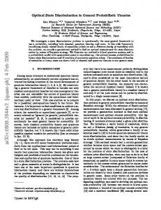
Table 1: SBCN main characteristics. Dataset Adult German credit Census-income
Figure 2: Distribution of edge scores. German credit: consists of 1000 tuples with 21 attributes on bank account holders applying for credit. The decision attribute is based on repayment history, i.e., whether the customer is labeled with good or bad credit risk. Also for this dataset the partial order for temporal priority has four orders. Personal attributes such as gender, age, foreign worker are defined in the first level. Personal attributes such as employment status and job status are defined in the second level. Personal properties such as savings status and credit history are defined in the third level, and finally the decision attribute is the last level. Census-income: consists of 299,285 tuples and 40 attributes, where each tuple correspond to an individual and it is described by demographic and employment attributes such as age, sex, relationship, education, employment, ext. Similar to Adult dataset, the decision attribute is the income levels and we define four levels in the partial order for temporal priority. Building the SBCN just take a handful of seconds in German credit and Adult, and few minutes in Census-income on a commodity laptop. The main characteristics of the extracted SBCN are reported in Table 1, while the distribution of the edges scores W (e) is plotted in Figure 2. As discussed in the Introduction we also use the dataset from the famous 1973 episode at University of California at Berkeley, in order to highlight the differences between correlation-based and causation-based methods. Berkeley Admissions Data: consists of 4,486 tuples and three attributes, where each tuple correspond to an individual and it is described by the gender of applicants and the department that they apply for it. For this dataset the partial order for temporal priority has three orders. Gender is defined in the first level, department in the second level, and finally the decision attribute is the last level. Table 2 is a three-way table that presents admissions data at the University of California, Berkeley in 1973 according to the variables department (A, B, C, D, E), gender (male, female), and outcome (admitted, denied). The table is adapted from data in the text by Freedman, et al. [34].
Community detection on the SBCN Given that our SBCN is a directed graph with edge weight, as a first characterization we try to partition it using a random-walks-based community detection algorithm, called Walktrap and proposed in [33], whose unique parameter is the maximum number of steps in a random walk (we set it to 8), and which automatically identifies the right number of communities. The idea is that short random walks tend to stay in the same community (densely connected area of the graph). Using this algorithm over the reconstructed SBCN from Adult dataset, we obtain 5 communities: two larger ones and three smaller ones (reported in Table 3). Interestingly, the two larger communities seem built around the negative (C1 ) and the positive (C2 ) decisions. Figure 1 in Section 3 shows the subgraph of the SBCN corresponding to C2 (that we can call, the favoritism cluster): we note that such cluster also contains nodes such as sex Male, age old, relationship Husband. The other large community C1 , can be considered the discrimination cluster: beside the negative decision it contains other nodes representing disadvantaged groups such as sex Female, age young, race Black, marital status Never married. This good separability of the SBCN in the two main clusters of discrimination and favoritism, highlights the goodness of the causal structure captured by the SBCN. 5.2
Group discrimination and favoritism
We next focus on assessing the discrimination score ds− we defined in Section 4.1, as well as the average number of steps that the random walks take to reach the negative and positive decisions, denote as− (v) and as+ (v) respectively. Tables 4, 5 and 6 report the top-5 and bottom-5 nodes w.r.t. the discrimination score ds− , for datasets Adult, German and Census-income, respectively. The first and most important observation is that our discrimination score provides a very clear signal, with some disadvantaged groups having very high discrimination score (equal to 1 or very close), and similarly clear signals of favoritism, with groups having ds− (v) = 0, or equivalently ds+ (v) = 1. This is more clear in the Adult dataset, where the positive and negative decisions are artificially derived from the income attribute. In the German credit dataset, which is more realistic as the decision attribute is truly about credit, both discrimination and favoritism are less palpable. This is also due to the fact that German credit contains less proper causal relations, as reflected in the higher sparsity of the SBCN. A consequence of this sparsity is also that the random walks generally need more steps to reach one of the two decisions. In Censusincome dataset, we observe favoritism with respect to married and asian pacific individuals.
Table 3: Communities found in the SBCN extracted from the Adult dataset by Walktrap[33]. In the table the attributes are shortened as in parenthesis: age (ag), education (ed), marital status (ms), native country (nc), occupation (oc), race(ra), relationship (re), sex (sx), workclass (wc). C1 negative dec, wc:Private, ed:Some college, ed:Assoc acdm, ms:Never married, ms:Divorced, ms:Widowed, ms:Married AF spouse, oc:Sales, oc:Other service, oc:Priv house serv, re:Own child, re:Not in family, re:Wife, re:Unmarried, re:Other relative, ra:Black, oc:Armed Forces, oc:Handlers cleaners, oc:Tech support, oc:Transport moving, ed:7th 8th, ed:10th, ed:12th, ms:Separated, ed:HS grad,ed:11th, nc:Outlying US Guam USVI etc, nc:Haiti, ag:young, sx:Female, ra:Amer Indian Eskimo, nc:Trinadad Tobago, nc:Jamaica, oc:Machine op inspct, ms:Married spouse absent, oc:Adm clerical, C2 positive dec, oc:Prof specialty, wc:Self emp not inc, ms:Married civ spouse, oc:Craft repair,oc:Protective serv, re:Husband, ed:Prof school, wc:Self emp inc, ag:old , wc:Local gov, oc:Exec managerial, ed:Bachelors, ed:Assoc voc, ed:Masters, wc:Never worked, wc:State gov, ed:Doctorate, sx:Male, nc:India, nc:Cuba C3 oc:Farming fishing, wc:Without pay, nc:Mexico, nc:Canada, nc:Italy, nc:Guatemala, nc:El Salvador, ra:White, nc:Poland, ed:1st 4th, ed:9th,ed:Preschool, ed:5th 6th C4 nc:Iran, nc:Puerto Rico, nc:Dominican Republic, nc:Columbia, nc:Peru, nc:Nicaragua, ra:Other C5 nc:Philippines, nc:Cambodia, nc:China, nc:South, nc:Japan, nc:Taiwan, nc:Hong, nc:Laos, nc:Thailand, nc:Vietnam, ra:Asian Pac Islander
5.3
Genuine requirement
We next focus on genuine requirement (or explainable discrimination). Table 7 reports some examples of fraction of explainable discrimination (both positive and negative) on the Adult dataset. We can see how some fractions of discrimination against protected groups, can be “explained” by intermediate nodes such as having a low education profile, or a simple job. In the case these intermediate nodes are considered legally grounded, then one cannot easily file a discrimination claim. Similarly, we can observe that the favoritism towards groups such as married men, is explainable, to a large extent, by higher education and good working position, such as managerial or executive roles.
5.4
Subgroup and Individual Discrimination
We next turn our attention to subgroup and individual discrimination discovery. Here the problem is to assign a score of discrimination not to a single node (a group), but to multiple nodes (representing the attributes of an individual or a subgroup of citizens). In Section 4.4 we have introduced based on the PageRank of the positive and negative decision, ppr(δ + ) and ppr(δ − ) respectively, personalized on the nodes of interest. Figure 3 presents a scatter plot of ppr(δ + ) versus ppr(δ − ) for each individual in the German credit dataset. We can observe the perfect separation between individuals corresponding to a high personalized PageRank with respect to the positive decision, and those associated with a high personalized PageRank relative to the negative decision.
Table 4: Top-5 and bottom-5 groups by discrimination score ds− (v) in Adult dataset. ds− (v) 1 0.996 0.995 0.994 0.98
relationship Unmarried marital status Never married age Young race Black sex Female relationship Husband marital status Married civ spouse sex Male native country India age Old
Table 5: Top-5 and bottom-4 groups by discrimination score ds− (v) in German credit. We report only the bottom-4, because there are only 4 nodes in which ds+ (v) > ds− (v). ds− (v) 1 1 1 0.86 0.791
as− (v) 6.0 2.23 6.0 3.68 5.15
as+ (v) 4.0 5.0
ds− (v) 0 0.12 0.186 0.294
as− (v) 8.0 7.0 6.48
as+ (v) 2.39 4.4 3.34 4.4
residence since le 1d6 residence since gt 2d8 residence since from 1d6 le 2d2 age gt 52d6 personal status male single job unskilled resident personal status male mar or wid age le 30d2 personal status female div or sep or mar
Table 6: Top-5 and bottom-5 groups by discrimination score ds− (v) in Census-income dataset. MIGSAME Not in universe under 1 year old WKSWORK 94 5 inf AWKSTAT Not in labor force VETYN 0 5 20 5 MARSUPWT 3188 455 4277 98 AHGA Doctorate degreePhD EdD AMARITL Married A F spouse present AMJOCC Sales ARACE Asian or Pacific Islander VETYN 20 5 32 5
ds− (v) 0 0 0 0 0
ds− (v) 0.71 0.625 0.59 0.58 0.55
as− (v) 4.09 3.0 2.0 1.01 5.0
as− (v) -
as+ (v) 8.82 6.76 6.16 5.17 9.25
as+ (v) 3.07 4.49 2.0 6.47 5.89
Table 7: Fraction of explainable discrimination for some exemplar pair of nodes in the Adult dataset. Source node race Amer Indian Eskimo sex Female age Young relationship Unmarried race Black Source node relationship Husband sex Male native country Iran native country India age Old
Intermediate education HS grad occupation Other service occupation Other service education HS grad education 11th
f ed− (v) 0.481 0.310 0.193 0.107 0.083 f ed+ (v) 0.806 0.587 0.480 0.415 0.39
Such good separation is also reflected in the generalized discrimination score (Definition 4) that we obtain by combining ppr(δ + ) versus ppr(δ − ).
0.04
0.08
ppr(−)
0.022 0.018 0.014
ppr(−)
0.010
0.02 0.010
0.015
0.020
0.03
0.04
0.07
0.08
Figure 5: Individual discrimination: scatter plot of ppr(δ + ) versus ppr(δ − ) for each individual in the Adult dataset. Red dots are for age Young and blue dots are for age Old.
0.4
100 60
0.0
female young young female
0 20
Frequency
0.8
Figure 3: Scatter plot of ppr(δ + ) versus ppr(δ − ) for each individual in the German credit dataset.
0.06
ppr(+)
0.025
ppr(+)
0.05
0.4 0.4
0.5
0.6
0.6
0.7
0.7
0.8
t
0.8
0.3
0.5
0.4
gds−
old single male old single male
0.0
Figure 4: Individual discrimination: histogram representing the distribution of the values of the generalized discrimination score gds− for the population of the German credit dataset.
0.3 In Figure 4 we report the distribution of the generalized discrimination score gds− for the population of the German credit dataset: we can make a note of the clear separation between the two subgroups of the population. In the Adult dataset (Figure 5) we do not observe the same neat separation in two subgroups as in the German credit dataset, also due to the much larger number of points. Nevertheless, as expected, ppr(δ + ) and ppr(δ − ) still exhibit anticorrelation. In Figure 5 we also use colors to show two different groups: red dots are for age Young and blue dots are for age Old individuals. As expected we can see that the red dots are distributed more in the area of higher ppr(δ − ). The plots in Figure 6 have a threshold t ∈ [0, 1] on the X-axis, and the fraction of tuples having gds− () ≥ t on the Y-axis, and they show this for different subgroups. The first plot, from the Adult dataset, shows the group female, young, and young female. As we can see the individuals that are both young and female have a higher generalized discrimination score. Similarly, the second plot shows the groups old, single male, and old single male from the German credit dataset. Here we can observe much lower rates of discrimination with only 1/5 of the corresponding populations having gds− () ≥ 0.5, while in the previous plot it was more than 85%.
0.4
0.5
0.6
0.7
t Figure 6: Subgroup discrimination: plots reporting a threshold t ∈ [0, 1] on the X-axis, and the fraction of tuples having gds− () ≥ t on the Y-axis. The top plot is from Adult, while the bottom is from German credit.
5.5
Comparison with prior art
In this section, we discuss examples in which our causation-based method draws different conclusions from the correlation-based methods presented in [13, 14, 15] using the same datasets and the same protected groups 7 . The first example involves the foreign worker group from German Credit dataset, whose contingency table is reported in Figure 7. Following the approaches of [13, 14, 15] the foreign worker group results strongly discriminated. In fact Figure 7 shows an RD value (risk difference) of 0.244 which is considered a strong signal: in fact RD > 0 is already considered discrimination [15]. However, we can observe that the foreign worker group is per se not very significant, as it contains 963 tuples out of 7
We could not compare with [22] due to repeatability issues.
1000 total. In fact our causal approach does not detect any discrimination with respect to foreign worker which appears as a disconnected node in the SBCN. The second example is in the opposite direction. Consider the race black group from Adult dataset whose contingency table is shown in Figure 8. Our causality-based approach detects a very strong signal of discrimination (ds− () = 0.994), while the approaches of [13, 14, 15] fail to discover discrimination against black minority when the value of minimum support threshold used for extracting classification rules is more than 10%. On the other hand, when such minimum support threshold is kept lower, the number of extracted rules might be overwhelming. Finally, we turn our attention to the famous example of false-positive discrimination case happened at Berkeley in 1973, that we discussed in Section 1. Figure 9 presents the SBCN extracted by our approach from Berkeley Admission Data. Interestingly, we observe that there is no direct edge between node sex Female and Admission No. And sex Female is connected to node Admission No through nodes of Dep C, Dep D, Dep E, and Dep F, which are exactly the departments that have lower admission rate. By running our random walk-based methods over SBCN we obtain the value of 1 for the score of explainable discrimination confirming that apparent discrimination in this dataset is due the fact that women tended to apply to departments with lower rates of admission. Similarly, we observe that there is no direct edge between node sex Male and Admission Yes. And sex Male is connected to node Admission Yes through nodes of Dep A, and Dep B, which are exactly the departments that have higher admission rate. By running our random walk-based methods over SBCN we obtain the value of 1 for the score of explainable discrimination confirming that apparent favoritism towards men is due to the fact that men tended to apply to departments with higher rates of admission. However, following the approaches of [13, 14, 15], the contingency table shown in Figure 10 can be extracted from Berkeley Admission Data. As shown in Figure 10, the value of RD suggests a signal of discrimination versus women.
Figure 10: Contingency table for female in the Berkeley Admission Data dataset. This highlights once more the pitfalls of correlation-based approaches to discrimination detection and the need for a principled causal approach, as the one we propose in this paper.
6.
CONCLUSIONS
Discrimination discovery from databases is a fundamental task in understanding past and current trends of discrimination, in judicial dispute resolution in legal trials, in the validation of micro-data before they are publicly released. While discrimination is a causal phenomenon, and any discrimination claim requires to prove a causal relationship, the bulk of the literature on data mining methods for discrimination detection is based on correlation reasoning. In this paper, we propose a new discrimination discovery approach that is able to deal with different types of discrimination in a single unifying framework. It is the first discrimination detection method grounded in probabilistic causal theory. We define a method to extract a graph representing the causal structures found in the database, and then we propose several random-walk-based methods over the causal structures, addressing a range of different discrimination problems. Our experimental assessment confirmed the great flexibility of our proposal in tackling different aspects of the discrimination detection task, and doing so with very clean signals, clearly separating discrimination cases. Repeatability. Our software together with the datasets used in the experiments are available at http://bit.ly/ 1GizSIG.
[2] EU Legislation, “(a) race equality directive,2000/43/ec, 2000; (b) employment equality directive, 2000/78/ec, 2000; (c) equal treatment of persons, european parliament legislative resolution, 2009.” [3] S. R. Foster, “Causation in antidiscrimination law: Beyond intent versus impact,” Hous. L. Rev., vol. 41, p. 1469, 2004. [4] M. Dabady, R. M. Blank, C. F. Citro et al., Measuring racial discrimination. National Academies Press, 2004. [5] P. J. Bickel, E. A. Hammel, and J. W. O’Connell, “Sex bias in graduate admissions: Data from berkeley,” Science, vol. 187, no. 4175, 1975. [6] C. Hitchcock, “Probabilistic causation,” in The Stanford Encyclopedia of Philosophy, 2012. [7] P. Suppes, A probabilistic theory of causality. North-Holland Publishing Company, 1970. [8] G. Schwarz, “Estimating the dimension of a model,” Annals of Statistics, vol. 6, no. 2, pp. 461–464, 1978. [9] B. Custers, T. Calders, B. Schermer, and T. Zarsky, Discrimination and Privacy in the Information Society: Studies in Applied Philosophy, Epistemology and Rational Ethics. Springer, 2012, vol. 3. [10] A. Romei and S. Ruggieri, “A multidisciplinary survey on discrimination analysis,” The Knowledge Engineering Review, pp. 1–57, 2013. [11] S. Hajian and J. Domingo-Ferrer, “A methodology for direct and indirect discrimination prevention in data mining,” TKDE, 25(7), 2013. [12] F. Kamiran and T. Calders, “Data preprocessing techniques for classification without discrimination,” KAIS, 33(1), 2012. [13] D. Pedreshi, S. Ruggieri, and F. Turini, “Discrimination-aware data mining,” in KDD, 2008. [14] D. Pedreschi, S. Ruggieri, and F. Turini, “Measuring discrimination in socially-sensitive decision records.” in SDM, 2009. [15] S. Ruggieri, D. Pedreschi, and F. Turini, “Data mining for discrimination discovery,” TKDD, 4(2), 2010. [16] B. T. Luong, S. Ruggieri, and F. Turini, “k-nn as an implementation of situation testing for discrimination discovery and prevention,” in KDD, 2011. [17] I. Rorive, “Proving discrimination cases: The role of situation testing,” 2009. [18] I. Zliobaite, F. Kamiran, and T. Calders, “Handling conditional discrimination,” in ICDM, 2011.
[19] C. Dwork, M. Hardt, T. Pitassi, O. Reingold, and R. Zemel, “Fairness through awareness,” in ITCS, 2012. [20] D. Pedreschi, S. Ruggieri, and F. Turini, “Integrating induction and deduction for finding evidence of discrimination,” in ICAIL, 2009. [21] S. Ruggieri, S. Hajian, F. Kamiran and X. Zhang, “Anti-discrimination Analysis Using Privacy Attack Strategies,” in PKDD, 2014. [22] K. Mancuhan and C. Clifton, “Combating discrimination using bayesian networks,” Artificial Intelligence and Law, 22(2), 2014. [23] D. Koller and N. Friedman, Probabilistic graphical models: principles and techniques. MIT press, 2009. [24] P. Menzies, “Counterfactual theories of causation,” in The Stanford Encyclopedia of Philosophy, spring 2014 ed., E. N. Zalta, Ed., 2014. [25] J. Woodward, “Causation and manipulability,” in The Stanford Encyclopedia of Philosophy, winter 2013 ed., E. N. Zalta, Ed., 2013. [26] E. Brenner and D. Sontag, “Sparsityboost: A new scoring function for learning bayesian network structure,” arXiv:1309.6820, 2013. [27] L. O. Loohuis, G. Caravagna, A. Graudenzi, D. Ramazzotti, G. Mauri, M. Antoniotti, and B. Mishra, “Inferring tree causal models of cancer progression with probability raising,” PLoS ONE, 9(12), 2014. [28] D. Ramazzotti et al. “Capri: Efficient inference of cancer progression models from cross-sectional data,” Bioinformatics, 31(18), 2015. [29] US Federal Legislation, “(a) equal credit opportunity act, (b) fair housing act, (c) intentional employment discrimination, (d) equal pay act, (e) pregnancy discrimination act, (f) civil right act., 2010.” [30] E. Ellis and P. Watson, EU anti-discrimination law. Oxford University Press, 2012. [31] S. Hajian, J. Domingo-Ferrer, A. Monreale, D. Pedreschi, and F. Giannotti, “Discrimination-and privacy-aware patterns,” DAMI, 29(6), 2015. [32] G. Jeh and J. Widom, “Scaling personalized web search,” in WWW 2003. [33] P. Pons and M. Latapy, “Computing communities in large networks using random walks,” in ISCIS, 2005. [34] D. Feedman, R. Pisani, and R. Purves, “Statistics,” 3rd Edition, WW Norton & Company, New York (1998).