arXiv:1401.7910v1 [cond-mat.stat-mech] 30 Jan 2014
Expressing the entropy of lattice systems as sums of conditional entropies. Torbjørn Helvik and Kristian Lindgren∗ Complex systems group, Department of Energy and Environment, Chalmers University of Technology, SE-41296 Göteborg, Sweden January 31, 2014
Abstract Whether a system is to be considered complex or not depends on how one searches for correlations. We propose a general scheme for calculation of entropies in lattice systems that has high flexibility in how correlations are successively taken into account. Compared to the traditional approach for estimating the entropy density, in which successive approximations builds on step-wise extensions of blocks of symbols, we show that one can take larger steps when collecting the statistics necessary to calculate the entropy density of the system. In one dimension this means that, instead of a single sweep over the system in which states are read sequentially, one take several sweeps with larger steps so that eventually the whole lattice is covered. This means that the information in correlations is captured in a different way, and in some situations this will lead to a considerably much faster convergence of the entropy density estimate as a function of the size of the configurations used in the estimate. The formalism is exemplified with both an example of a free energy minimisation scheme for the two-dimensional Ising model, and an example of increasingly complex spatial correlations generated by the time evolution of elementary cellular automaton rule 60.
1
Introduction
Many models in statistical mechanics involve a lattice of particles having spins or other states from a finite set, and with interaction between neighboring particles defined by a transition invariant potential. The Ising model, which was solved by Onsager in 1944 [19], epitomizes such models. An important problem is to find the entropy density of the Gibbs state corresponding to the interaction potential. This and other properties of lattice models are often investigated by Monte Carlo relaxation methods such as the Metropolis algorithm. These methods yields estimates of thermodynamic quantities that can be directly measured in ∗
[email protected]
1
simulation runs, such as internal energy u and long range order. However, neither the entropy density s nor the free energy f = u − T s can be obtained directly, so special approaches are needed. Several methods have been devised to estimate the entropy of lattice systems using MC simulations, the most important one being thermodynamic integration. See [2] for a review. We will in this paper be concerned with how the entropy density can be written in terms of sums of appropriate conditional entropies of spin variables. The method is not confined to finding entropies of Gibbs states, but can be applied to any probability measure on lattice systems in any dimension. The first person which, to our knowledge, used conditional entropies to investigate two-dimensional lattice systems was Alexandrowicz [1]. His approach was to generate lattice configurations by adding spins one by one to an empty lattice using a Markov process. The transition probabilities of the process was parameterized and depended on previous spins in some neighborhood. The best parameter values was found for each inverse temperature β by optimizing according to the minimum free energy principle. Entropy was then estimated as the average of log p1 , with p being the probability of the realized transition. This is tantamount to estimating the conditional entropy of a spin with respect to the spins in some neighborhood. In [14] Meirovitch introduced the idea that instead of searching for optimal transition probabilities, the transition probabilities could be directly estimated from looking at frequencies in a lattice configuration obtained, e.g., from a Monte Carlo algorithm. In [21, 22] Schlijper et. al. combined this method of calculating entropy with the Cluster Variation Method [20] to obtain both a lower bound and an upper bound on the entropy. They also put the method on formal ground, in particular using a result on the global Markov property for spin systems [5]. The method of using empirical frequencies for estimating the entropy has several advantages. It is cost effective and can easily be included into a MC algorithm to monitor the entropy and free energy during a MC simulation. The method basically needs only a single lattice configuration and is easily adaptable to more involved problems. Schlijper et. al., and also Alexandrowicz, pointed out that for a lattice configuration fluctuations in energy and entropy tend to cancel. As a consequence of this, free energy, which often is the interesting quantity, is more easily determined than its separate contributions entropy and energy. The effectivity of the method has been demonstrated by both Meirovitch and Schlijper et. al, and it has been used in several applications, e.g., [13, 15, 16, 17, 18]. An approach based on conditional entropies usually means that one searches for correlations, and the more information that is found in correlations the less is the estimate of the entropy. This search for correlations typically involves extensions of blocks in a regular way: In one dimension, one uses entropies conditioned on an increasing sequence of lattice sites to the left. In two dimensions, one may extend a rectangular block in a similar way forming conditional entropies, or, alternatively one may extend blocks one lattice site at the time using a lexicographic ordering, as was exploited already by Kramers and Wannier [9]. How well this approach works for estimating the entropy depends on convergence properties of the conditional entropies, reflecting how long correlations that are present in the system and how they decline with distance. In a complex system, correlations may not be so easily detected, and it may turn out 2
that the traditional approach, extending blocks by adding neighbouring lattice sites, is not efficient. Instead one may consider a search for correlations in which larger steps are taken, temporally disregarding states in lattice sites in-between, which is an approach we present here. The main contribution of this paper is a general and flexible scheme for obtaining representations of the entropy density of a lattice system in terms of suitable sums of conditional entropies. This is achieved by scanning the lattice in the order suggested by some regular sublattice, and possibly multiple times in succession. Our results adds flexibility to the empirical frequency approach to estimating entropy. We present the procedure for general point lattices in Section 2. In Section 3, we discuss how the procedure can be helpful in finding simple expressions when the measure is a Gibbs state with finite interaction range, and this is exemplified by an entropy estimate applied to the two-dimensional Ising model. In Section 4, we show how the main theorem can be used to create a hierarchical decomposition of the entropy, and this is illustrated with entropy estimates of patterns generated by elementary cellular automaton rule 60. The result on representations of entropy densities are also related to several information theoretic notions of structure and complexity in lattice systems. This includes the effective measure complexity introduced by Grassberger [6], the excess entropy [4], and local information introduced for one dimensional systems in [7]. Whether a system is considered complex or not depends on how one searches for correlations – a clever scheme for scanning the lattice may reveal structure that would not be so easily detected using a traditional approach.
2 2.1
Entropy density in Point lattices Background
By the term lattice we mean a regularly spaced array of points in Rd . The correct mathematical term is point lattice, as the term lattice is a more general structure. Formally, a point lattice V is a a discrete abelian subgroup of Rd . Typical point lattices in R2 are the quadratic grid and the hexagonal lattice. The triangular lattice is actually a union of two point lattices which are translates of each other by a constant. We will use the term lattice in this paper to refer to the union of a finite number translations of a single point lattice V . We will first present our result, Theorem 1, for a single lattice. We then discuss how it can be extended to a general union of translates of a point lattice. When drawing a lattice V ⊂ Rd it is convenient to draw the corresponding Voronoi cells instead. The Voronoi cell of v ∈ V is the subset {x ∈ Rd : |x − v| < |x − u| ∀ u ∈ V, v 6= u}. The collection of all Voronoi cells comprises a periodic tiling of Rd . Se Fig. 1 for illustrations. We now consider spin systems on a point lattice V . By this we mean that each lattice point represents a particle which has some spin from a finite set A. We first introduce some terminology. Let V be a point lattice. For guiding the intuition, it can be useful to think of V as Zd or just the grid Z2 . The point lattice is represented by an ordered collection e1 , . . . , ed of linearly independent unit vectors in Rd such that ( d ) X V = he1 , . . . , ed i = v i e i : vi ∈ Z . i=1
3
a.
b.
c.
Figure 1: Lattices in R2 with corresponding Voronoi cells. a. Cubic, b. Hexagonal, c. Triangular. The representation of a point v ∈ V in terms of (v1 , . . . , vd ) is unique. Note that 0 ∈ V for any point lattice V . For two subsets Λ, Λ0 ⊂ V of the point lattice, write Λ + Λ0 = {v + v 0 : v ∈ Λ, v 0 ∈ Λ0 } . Define the unit d-cube as Ud = {v ∈ V : sup1≤i≤d |vi | ≤ 1}, and define the boundary of a set Λ ⊂ V as ∂Λ = Λ ∩ (Ud + ΛC ) . We say that Λn ↑ V in the van Hove sense if S 1. n Λn = V , 2. Λn ⊂ Λn+1 ∀n, 3. limn→∞ |∂Λn |/|Λn | = 0. e1 , . . . , eˆm i of the lattice is the collection PAn m-dimensional subgroup G = hˆ { i gi eˆi } of all linear combinations of a set of m linearly independent vectors eˆ1 , . . . , eˆm ∈ V . The subgroup is itself a point lattice. We define a tiling1 of V as follows. Definition 1. A tiling of a d-dimensional point lattice V is a pair (A, G) consisting of a finite subset A ⊂ V with 0 ∈ A and a d-dimensional subgroup G of V satisfying 1. A + G = V . T 2. (A + g) (A + h) = ∅ for all g, h ∈ G, g 6= h. P We willPuse the lexicographical order on G. For g, g 0 ∈ G, write g = i gi eˆi and g 0 = i gi0 eˆi . We say that g < g 0 if there is an i, 1 ≤ i ≤ k, such that gi < gi0 and gj = gj0 for j < i. Note that due to the use of the lexicographical order, we do not consider, e.g., the tiling of V = Z2 with A = {(0, 0)} and G = h(1, 0), (0, 1)i and the tiling with A = {(0, 0)} and G = h(1, 0), (1, 1)i as equal. Based on the lexicographical order, we define the subset G− ⊂ G as G− = {g ∈ G : g < 0}. An example of a tiling of the 2-dimensional square lattice is illustrated in Fig. (2). 1 This
is a non-standard use of the term tiling.
4
Figure 2: Example of a tiling of the square lattice. The tiling is defined by (A, G) with A = {(0, 0), (0, 1), (0, 2)} and G = h(1, 1), (1, −2)i. The set A is marked with a thick line and the sub lattice G− is shaded.
2.2
Measures and entropy
Let A be a finite set consisting of the possible spins and let Λ ⊆ V . An assignment of a spin in A to each element of Λ is called a configuration of Λ. We denote a configuration of Λ by xΛ . The set of all configurations of Λ is denoted by AΛ . A configuration xV on the entire space will be denoted just by x. Let the set M consist of all translation invariant probability measures on AV . These are often called states in statistical mechanics. The restriction of a measure µ ∈ M to AΛ is denoted by µΛ . We drop the subscript when no confusion can occur. A translation invariant measure is uniquely defined by specifying its restriction to all finite Λ ∈ V . The entropy of a subset Λ with respect to a measure µ is defined as X S(Λ) = − µΛ (xΛ ) log µΛ (xΛ ) . (1) xΛ ∈AΛ
The entropy is the average information that is gained by observing the configuration on Λ, where information is used in the sense of Shannon [23]. The entropy density of a measure µ is defined as the average entropy per spin. That is, as the limit sµ = lim
n→∞
1 S(Λn ), |Λn |
(2)
where Λn ↑ V in the van Hove sense. It is well known that s also can be written as a conditional entropy. Let Λ and Λ0 be finite subsets of V . The conditional entropy of Λ given Λ0 with respect to µ is defined as X S(Λ|Λ0 ) = − µ(xΛ∪Λ0 ) log µ(xΛ |xΛ0 ), (3) xΛ∪Λ0
where µ(xΛ |xΛ0 ) = µ(xΛ∪Λ0 )/µ(xΛ ). This is the information gained from observing the configuration on Λ when the configuration on Λ0 is known. 0 PFor Λ infinite, the conditional entropy is defined by a limit. Define Vn = { i vi ei : |vi | ≤ n ∀ i}, and S(Λ|Λ0 ) = lim S(Λ|Λ0 ∩ Vn ) . n→∞
(4)
Convergence is ensured by the monotonicity property of conditional entropy: 5
Lemma 1. Λ0 ⊆ Λ00 ⇒ S(Λ|Λ00 ) ≤ S(Λ|Λ0 ) . Proof. When Λ0 ⊆ Λ00 we have S(Λ|Λ0 ) − S(Λ|Λ00 ) =
X
µ(xΛ∪Λ00 ) log
µ(xΛ |xΛ00 ) = µ(xΛ |xΛ0 )
X
µ(xΛ |xΛ00 ) log
xΛ∪Λ00
=
X
µ(xΛ00 \Λ )
xΛ00 \Λ
xΛ
µ(xΛ |xΛ00 ) ≥ 0, µ(xΛ |xΛ0 )
where the inequality follows from the fact that the second sum is the KullbackLeibler divergence, or the relative entropy, between the distributions µ(xΛ |xΛ0 ) and µ(xΛ |xΛ00 ), which is a non-negative quantity [10]. This concludes the proof. A further consequence of this result is that conditional entropy is bounded above by log |A| per spin. S(Λ|Λ0 ) ≤ S(Λ) ≤ |Λ| log |A| . (5) For a one-dimensional lattice it is easy to prove that sµ = S({0}|{i : i < 0}) [3]. It is practical to represent the expression graphically in the following way sµ =
(6)
The right hand side is to be interpreted as the conditional entropy of the spin at the cross conditioned on the spins all filled cells (which here are all spins to the left). This representation of the expression will prove useful later, when the situation is more involved. Before we proceed to the main result we state a simple but very useful property of conditional entropies that follows from (3). Observation 1. For finite Λ, Λ0 , Λ00 ⊂ V , S(Λ ∪ Λ0 |Λ00 ) = S(Λ|Λ0 ∪ Λ00 ) + S(Λ0 |Λ00 ) .
(7)
Also note that for a translation invariant measure µ on AV , S(Λ|Λ0 ) = S(Λ + v|Λ0 + v) ∀ v ∈ V .
2.3
Main result
The main result of this paper shows that there is great flexibility in choosing how to express the entropy density in terms of conditional entropies. The various expressions are achieved through using different tilings of V and coverings of the basic tile A. The method is applicable in all dimensions d. Theorem 1. Let V be a point lattice in Rd and let µ be a translation invariant measure on AV . Let (A, G) be a tiling of V . Partition A into N nonempty sets Sk−1 A1 , . . . , AN , with 1 ≤ N ≤ |A|. Define A