sis, control and recognition using statistical active facial ap- pearance models for face analysis [7]. 2 Active facial appearance models. 2.1 Model description.
Expressive face recognition and synthesis Bouchra Abboud, Franck Davoine, Mˆo Dang Heudiasyc Laboratory. CNRS, University of Technology of Compi`egne. BP 20529, 60205 COMPIEGNE Cedex, FRANCE.
Abstract
nearly all cultures, facial expressions of six basic emotional categories are universally recognized, namely: joy, sadness, anger, disgust, fear and surprise [2]. Several other emotions and many combinations of emotions have been studied but remain unconfirmed as universally distinguishable. Thus, most of the research up to now has been oriented towards detecting these six universal expressions [3, 4, 5, 6]. In this paper we will address the issue of face tracking, video realistic face generation and facial expression synthesis, control and recognition using statistical active facial appearance models for face analysis [7].
Facial expression interpretation, recognition and analysis is a key issue in visual communication and man to machine interaction. In this paper, we present a technique for extracting appearance parameters from a natural image or video sequence, which allow reproduction of natural looking expressive synthetic faces. This technique was used to perform face synthesis and tracking in video sequences as well as facial expression recognition and control.
1 Introduction
2 Active facial appearance models
Natural human-machine interaction is becoming an active and important research area. Adequate feedback like speech, facial expression and body gestures is an essential component of such interaction since these communicative events satisfy certain communication expectations in human-human interaction. Furthermore, there has been an increased interest in the last years in trying to introduce human to human communication modalities into humancomputer interaction. This includes a number of approaches like speech recognition, eye tracking, data fusion and emotion understanding through facial expression recognition. Consistent machine interaction with the received and processed multi-modal stimuli will be conveyed through a photo-realistic virtual face, voice, body and gestures in order to simulate a humane machine. Possible applications are tourism, cultural heritage, eCommerce, technology enhanced learning, multimedia production, handicap, cognitive robots, vehicle on-board safety systems, etc. The human face comprises major information about identity and emotion. It constitutes a source of many informative social signs [1] and improves the response to communication expectations. For instance, lip-reading helps to understand speech, gaze patterns as well as head gestures like nodding or frowning direct the attention and regulate the conversation, whereas facial expressions communicate information about the feelings or mental states of other dialogue participants. Regarding emotions, previous works showed that in
2.1 Model description It has been shown that the active appearance model [7] is a powerful tool for face synthesis and tracking. It uses Principal Component Analysis to model both shape and texture variations seen in a training set of visual objects. After com� and aligning all shapes from the puting the mean shape � training set by means of a Procrustes analysis, the statistical shape model is given by:
�� � �� � �� ���
(1)
�� � �� � �� ���
(2)
where �� is the synthesized shape, � � is a truncated matrix describing the principal modes of shape variations in the training set and � �� is a vector that controls the synthesized shape. It is then possible to warp textures from the training set � in order to obtain shape-free of faces onto the mean shape � textures. Similarly, after computing the mean shape-free � and normalizing all textures from the training set texture � relatively to � � by scaling and offset of the luminance values, the statistical texture model is given by: where �� is the synthesized shape-free texture, � � is a truncated matrix describing the principal modes of texture variations in the training set and � �� is a vector that controls the synthesized shape-free texture. 1
By combining the training shape and texture vectors � �� and ��� and applying further PCA the statistical appearance model is given by:
�� � �� � �� ��
(3)
�� � �� � �� ��
(4)
a
b
c
Figure 1: a: Target (original face). b: Model initialization. c: Iterative model refinement until convergence to the target face.
where �� and �� are truncated matrices describing the principal modes of combined appearance variations in the training set, and �� is a vector of appearance parameters simultaneously controling both shape and texture. Given the parameter vector � � , the corresponding shape �� and shape-free texture � � can be computed respectively using equations (3) and (4). The reconstructed shape-free texture is then warped onto the reconstructed shape in order to obtain the full appearance of a face. Furthermore, in order to allow pose displacement of the model, it is necessary to add to the appearance parameter vector � � a pose parameter vector � � allowing control of scale, orientation and position of the synthesized face. While a couple of appearance parameter vector � and pose parameter vector � represents a face, the active appearance model can automatically adjust those parameters to a target face [8], by minimizing a residual image ���� �� which is the texture difference between the synthesized face and the corresponding mask of the image it covers. For this purpose, a set of training residual images are computed by displacing the appearance and pose parameters whithin allowable limits. These residuals are then used to compute matrices �� and �� establishing the linear relationships Æ��� � ��� ���� �� and Æ��� � ��� ���� �� between the parameter displacements and the corresponding residuals, so as to minimize ������ �� � Æ ��� ����¾ . An iterative model refinement procedure [8] is then used to drive the appearance model towards the actual face in the image.
Figure 2: Upper row : original unseen faces. Lower row: reconstructed synthetic faces inserted onto the original ones (the shape of the facial mask represented by the model is illustrated by the set of white points). We selected 338 frontal still face images composed of 26 neutral expression faces, 26 moderate and 26 high magnitude anger, disgust, fear, joy, surprise and sadness expressions. Each moderate expression image has been chosen manually by extracting an intermediate frame from the video sequence. In order to build the model, a shape � of 57 landmarks is manually positioned on each of the 338 images, yielding shape-free texture vectors � of 3493 pixels. The model is built using 50 shape modes, 150 texture modes and 40 appearance modes: the vector � is composed of 40 components, that retain 98 percent of the combined shape and texture variation. The shape-free texture vector � is composed of 3493 pixels. The active appearance search algorithm is illustrated on a previously unseen face (figure 1.a) with the mean shape and texture used as a first approximation (figure 1.b). The model output converges to the target face as shown in figure 1.c.
In the following, the appearance and pose parameters obtained by this optimization procedure will be denoted respectively as ��� and ��� .
2.2 Experimental setup The appearance model is built using the CMU expressive face database [9]. Each sequence of this database contains ten to twenty images, beginning with a neutral expression and ending with a high magnitude expression. 2
where �� · ½ is the pseudo inverse of � � ½ . The information relative to the person’s identity will then be retrieved by filtering out the expression information contained in vector �� ����� �, the latter being evaluated at the estimated expression intensity ���� using equation (6). This gives the identity vector ���� : ���� � ��� � �� ����� � (8)
Three other adaptations of a higher resolution appearance model computed on the same learning set are shown on figure 2.
3 Facial expression analysis/synthesis 3.1 Facial expression modeling
Having this, it is possible to modify the facial expression intensity represented in vector � � ����� � by modifying the � value in equation (6). In particular it is possible to filter out the expression by setting � � �.
The aim of this section is to study a linear model, as it is proposed in [10, 11]. In the same way as Cootes et al. [10] modeled the facial appearance parameters as a linear function of the orientation, Kang et al. [11] propose a linear model that correlates the appearance parameters to facial expression intensity according to:
� � �� ¼ � �� ½ � � �
�� ��� � �� ¼ � �� ½ � � � �� ¼
(9)
Then by adding the identity vector � ��� to the corrected expression it is possible to modify the expression intensity shown on the target face from high magnitude to neutral as shown in figure 3c:
(5)
where � is a scalar varying from � � � to indicate neutral expression to � � � to indicate a high magnitude expression and � is the approximation error. � � ¼ and �� ½ are coefficient vectors learnt for each facial expression ( is joy, fear, disgust, surprise, fear, sadness or neutral) by linear regression over the training set. The linear regression is performed using 3 control points for each expression namely neutral expression (� � �), moderate expression (� � ���) and high magnitude expression (� � �).
� � ����
� �� ��� � � �
(10)
���
3.2 Facial expression filtering Once the coefficient vectors � � ¼ and �� ½ have been learnt for a given expression , the linear model can be used to predict an artificial vector of appearance parameters � � ��� for a given intensity � of the expression :
�� ��� � �� ¼ � �� ½ �
a
� �� ·½ �� � �� ¼ � ��
c
Figure 3: a: Target (original face). b: Reconstructed face using ��� obtained by iterative model adjustment to target face. c: Neutral expression obtained by canceling joy intensity.
(6)
Note that a given intensity � of the expression generates an unique value of the vector � � ���: the latter encodes thus an average appearance of this expression intensity, independently of any particular person. This means that the information about identity is contained in the residual � in equation 5. Therefore, in order to synthesize a new expression intensity �� for a given person, the residual for this person has to be added to the average appearance � � ��� � of this new intensity. The procedure for doing this is detailed below. Starting from an unseen face with a given expression (Fig. 3a), an appearance parameter vector � �� is first estimated as described at the end of 2.1, so that � �� synthesizes an artificial face similar to this target face (Fig. 3b). Having a priori knowledge of the facial expression represented on the target face, it is then possible to estimate the intensity of this expression by inverting equation (6): ����
b
3.3 Facial expression synthesis Starting from the artificially generated neutral expression of the target face, it is possible to artificially generate any desired expression � by applying the same method described in 3.2. It is assumed that the linear model (5) for the new expression � has been learnt on the training set, giving the corresponding � �¼ ¼ and ��¼ ½ parameters. In the procedure described above, the appearance parameters describing the target face ��� will now be replaced by � � ���� . It is then possible to estimate the intensity of the desired expression on the artificial neutral face. This value should be close to zero. ����� � ��¼ · (11) ½ �� � ���� � ��¼ ¼ ��
(7) 3
The estimated expression information vector at the � ���� intensity of the desired expression is given by:
�� ����� � � �� ¼ � �� ½ ���� � ¼
�
¼
�
¼
(12)
The new residual � ��� is then given by:
���� � � � ���� � �� ����� �� ¼
�
(13)
The facial expression intensity represented in vector
�� ����� � can be controlled through the parameter � in equa¼
�
tion (6). In particular it is possible to generate a high magnitude expression parameter estimation by setting � � �. Then by adding the identity vector � ��� to the corrected expression estimation vector � �¼ ������ � it is possible to modify the expression intensity shown on the target face from neutral to high magnitude as shown in figure 4.
�� �� ��
� �� ��� � � � ¼
(14)
���
Figure 5: Upper row : original surprised face. Middle row: synthetic expressive face inserted onto the original one. The appearance model may be used to track the face expression in a video. Lower row: synthetic expressive face linearly predicted using eq. 6
a
b
c
d
e
f
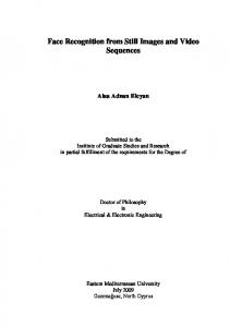
��� parameter vector allows to estimate the facial expression intensity ���� using equation (7), as well as the linearly predicted vector of appearance parameters � � ����� � at this intensity. For each facial expression, the � � ����� � parameters tend to follow a well defined trajectory whose behavior can be linearly approximated by the linear model computed in section 3.1. This is illustrated in figure 6 showing the evolution of the first variation mode (first coefficient of � � ����� �) over 15 video sequences on each sequence, the face displays an expression going from neutral to high magnitude, respectively for anger (left plot) and sadness (right plot).
Figure 4: Generation of six synthetic expressions starting from the expression filtered face of figure 3.c. a: Anger. b: Disgust. c: Fear. d: Joy. e: Surprise. f: Sadness
Sadness expression Mode 1
Anger expression Mode 1
3.4 Expression evolution over a video sequence
0.14
0.08
0.12
0.07
0.1
0.06
0.08
0.05 0.06
In order to analyze the temporal behaviour of the linear model obtained in section 3.1, a series of experiments has been performed on a set of 15 videos representing different persons showing a facial expression gradually evolving from neutral to high magnitude. The active appearance model is fit on each image of a video sequence , using the previous output of the model as a first approximation of appearance and pose parameters as shown on figure 5 (middle row). At each step of the video sequence, the obtained
0.04 0.04
0.03 0.02
0.02
0
−0.02
0
5
10
15
20
0.01
025
5
10
15
20
25
Figure 6: For anger and sadness, evolution of 1st mode of �� ����� � over each video sequence. Straight line: 1st mode of �� ���, with � linearly varying from 0 to 1.
4
4 Facial expression recognition neutral anger disgust fear joy surprise sadness
Automatic recognition of facial expressions has been studied in many previous works. Local representations have been used, such as graphs of 2D Gabor wavelet responses in Lyons et al. [4], or direction of motions computed from the optical flow as in Yacoob and Davies [12]. Global representations have also been much investigated: Donato et al. [3] review and compare holistic representations including eigenfaces, Fisherfaces, independent component analysis, applied on difference texture images or optical flow. Lien et al. [13] propose to recognize facial actions by modeling the temporal evolution of local features as a hidden Markov model. In this work, we study the discriminating power of the combined appearance parameter �. To classify a new face represented by the parameter vector � � , and assuming that the expression classes have a common covariance matrix, we measure the squared Mahalanobis distance � as shown in equation 15 from � � to each of the � estimated mean vector � � in the original space, and assign � � to the class of the nearest mean. � � [joy, fear, disgust, surprise, fear, sadness, neutral] and is the estimated common covariance matrix of the training set. We repeat the same procedure within a Linear Discriminant Analysis subspace [14], and we measure the squared Mahalanobis distance � ��� as shown in equation 16, where � ��� is the projection of the � �� vector on the LDA space, ����� is the � estimated mean
vector in the LDA space and ��� is the estimated common covariance matrix of the projected training set. Finally we to the class of the nearest mean. assign ���� �
� �� � �� � � �� � �� � ½ �� � �� �
�
�
�
�
�
� �� � �� � � �� � �� � ½ �� � �� � ���
��� �
���
��� �
��� �
�
���
��� �
���
neutral anger disgust fear joy surprise sadness
neut. 38 1 0 0 0 1 3
ang. 1 10 0 0 0 0 0
disg. 1 0 12 1 0 0 0
fea. 4 0 0 8 2 0 0
joy 0 0 0 0 11 0 0
surp. 0 0 0 0 0 13 0
disg. 0 0 11 0 0 0 0
fea. 4 0 0 7 0 0 0
joy 0 0 0 0 13 0 0
surp. 0 0 0 0 0 13 0
sad. 7 1 0 0 0 2 6
neut. 35 3 1 3 0 0 3
ang. 4 7 1 0 0 0 2
disg. 2 2 10 0 1 0 0
fea. 4 0 0 4 2 1 1
joy 0 0 0 1 10 0 0
surp. 0 0 0 0 0 14 0
sad. 7 0 0 1 0 0 11
Table 3: Confusion matrix, for a nearest neighbor classifier in the original space, using 130 unknown test images.
neutral anger disgust fear joy surprise sadness
(16)
neut. 29 1 0 0 0 0 2
ang. 1 10 1 0 0 0 3
disg. 1 0 10 1 0 0 0
fea. 5 0 1 7 1 1 0
joy 1 0 0 0 12 0 0
surp. 0 0 0 0 0 13 0
sad. 15 1 0 1 0 1 12
Table 4: Confusion matrix, for a nearest neighbor classifier in the LDA space, using 130 unknown test images.
We also use a nearest neighbor classification scheme in the original and LDA spaces using the Mahalanobis distances � and ���� . Results are shown in tables 1 to 4. Percentages of good classifications of each facial expression for the different schemes are shown in table 5 for comparison.
neutral anger disgust fear joy surprise sadness
ang. 1 10 1 0 0 0 2
Table 2: Confusion matrix for the Mahalanobis distance expression classifier in the LDA space, using 130 unknown test images.
(15)
neut. 40 2 0 2 0 2 9
�
�
73.1 83.3 100 88.9 84.6 86.7 82.3 81.5
76.9 83.3 91.7 77.8 100 86.7 35.3 76.9
neutral anger disgust fear joy surprise sadness total
sad. 8 1 0 0 0 1 14
���
�
67.3 58.3 83.3 44.4 76.9 93.3 64.7 70.0
�
���
55.8 83.3 83.3 77.8 92.3 86.7 70.6 71.5
Table 5: Percentages of good classification of all facial expressions for different classification schemes in the original and LDA spaces using 130 test images.
Table 1: Confusion matrix for the Mahalanobis distance expression classifier in the original space, using 130 unknown test images.
The LDA subspace is computed so as to maximize class separability, and allows thus an optimal visualization of the 5
class structure. In Figure 7, the classes appear indeed much better separated in the LDA space than in the original space; that is reflected in the greatly increased value of Fisher criterion ������ �� . The “sad” expression appears poorly separated from the other classes, especially from the neutral class, which explains the worse classification rates for this class.
0.3
0.2
0.1
LDA space
[6] B. Fasel and J. Luettin, “Automatic facial expression analysis: a survey,” Tech. Rep. RR 99-19, IDIAP, Martigny, Valais, Switzerland, Dec. 2000.
Neutral Anger Disgust Fear Joy Surprise Sadness
0.15
0.1
0.05
[7] T.F. Cootes, G.J. Edwards, and C.J. Taylor, “Active appearance models,” IEEE Transactions on Pattern Analysis and Machine Intelligence, vol. 23, no. 6, pp. 681–685, June 2001.
C
2
C2
0
Neutral Initial space Anger Disgust Fear Joy Surprise Sadness
[5] M. Pantic and L.J.M. Rothkrantz, “Automatic analysis of facial expressions: The state of the art,” IEEE Transactions on Pattern Analysis and Machine Intelligence, vol. 22, no. 12, pp. 1424–1445, December 2000.
−0.1 0
−0.2
[8] T.F. Cootes and P. Kittipanya-ngam, “Comparing variations on the active appearance model algorithm,” in British Machine Vision Conference, Cardiff University, September 2002, pp. 837–846.
−0.05
−0.3
−0.4 −0.5
−0.4
−0.3
−0.2
C1
−0.1
0
0.1
−0.1 0.2 −0.1
−0.05
0
0.05
C1
0.1
0.15
0.2
0.25
Figure 7: 2D representation of the first 2 modes of the training set. Left: In the original space with Fischer criterion value ������ �� � �� . Right: Projected in the LDA space with Fischer criterion value
��� �
��� �
[9] T. Kanade, J. Cohn, and Y.L. Tian, “Comprehensive database for facial expression analysis,” in International Conference on Automatic Face and Gesture Recognition, Grenoble, France, March 2000, pp. 46– 53.
� ��� �.
[10] T.F. Cootes, K. Walker, and C.J. Taylor, “View-based active appearance models,” in International Conference on Automatic Face and Gesture Recognition, Grenoble, France, March 2000, pp. 227–232.
5 Conclusion and perspectives In this paper, we have presented different applications of Active Appearance Models for expressive face synthesis and recognition. We are currently investigating other classification approaches, based on linear or non-linear schemes. In addition to the greylevel texture, edges, multi-resolution Gabor responses, or color [15] could also be exploited to perform facial expression recognition.
[11] H. Kang, T.F. Cootes, and C.J. Taylor, “Face expression detection and synthesis using statistical models of appearance,” in Measuring Behavior, Amsterdam, The Netherlands, August 2002, pp. 126–128. [12] Y. Yacoob and L. Davis, “Recognizing facial expressions by spatio-temporal analysis,” in Proceedings of the International Conference on Pattern Recognition, Jerusalem Israel, October 1994, pp. 747–749.
References [1] V. Bruce and A. Young, In the eye of the beholder. The science of face perception, University Press, Oxford, 1998.
[13] Jenn-Jier James Lien, Takeo Kanade, Jeffrey Cohn, and C. Li, “Detection, tracking, and classification of subtle changes in facial expression,” Journal of Robotics and Autonomous Systems, vol. 31, pp. 131 – 146, 2000.
[2] P. Ekman, Facial Expressions, chapter 16 of Handbook of Cognition and Emotion, T. Dalgleish and M. Power, John Wiley � Sons Ltd., 1999.
[14] S. Dubuisson, F. Davoine, and M. Masson, “A solution for facial expression representation and recognition,” Signal Processing: Image Communication, vol. 17, no. 9, pp. 657–673, October 2002.
[3] G. Donato, M.S. Bartlett, J.C. Hager, P. Ekman, and T.J. Sejnowski, “Classifying facial actions,” IEEE Transactions on Pattern Analysis and Machine Intelligence, vol. 21, no. 10, pp. 974–988, October 1999.
[15] M.B. Stegman and R. Larsen, “Multi-band modelling of appearance,” in First International Workshop on Generative Model-Based Vision GMBV, Copenhagen Denmark, June 2002, pp. 101–106.
[4] M.J. Lyons, J. Budynek, and S. Akamatsu, “Automatic classification of single facial images,” IEEE Transactions on Pattern Analysis and Machine Intelligence, vol. 21, no. 12, pp. 1357–1362, December 1999. 6