Abstractâ A humanoid robot can be viewed as a constrained dynamic system with constraints imposed by manipulation tasks, locomotion tasks, and the ...
2015 IEEE International Conference on Robotics and Automation (ICRA) Washington State Convention Center Seattle, Washington, May 26-30, 2015
Extended Cooperative Task Space for Manipulation Tasks of Humanoid Robots H. Andy Park and C. S. George Lee Abstract— A humanoid robot can be viewed as a constrained dynamic system with constraints imposed by manipulation tasks, locomotion tasks, and the environment. This paper focuses on dealing with constraints in the upper-body of humanoid robots for manipulation tasks that involve coordinated motion of two arms. Inspired by research on human bimanual actions in the biomechanics area, we have developed the Extended-Cooperative-Task-Space (ECTS) representation that efficiently describes various coordinated motion tasks performed by a humanoid robot. Furthermore, we present a general whole-body control framework as an optimal controller based on Gauss’s principle of least constraint. We show that all the constraints imposed on a humanoid system can be handled in a unified manner. The proposed framework is verified by numerical simulations on a Hubo II+ humanoid robot model. Fig. 1. The CTS variables defined for two subsystems in a humanoid: upper-body and lower-body subsystems [1].
I. I NTRODUCTION Modeling and control of humanoid robots are quite challenging because of their large number of degrees-offreedom (DoF) and the task and environment constraints imposed on their movements. Thus, it is advantageous to view a humanoid robot in terms of two subsystems [1] – a manipulation subsystem (i.e., the upper-body subsystem) and a locomotion subsystem (i.e., the lower-body subsystem) as illustrated in Fig. 1. In this paper, we focus on the manipulation subsystem of humanoid robots and present a general framework by extending the Cooperative-TaskSpace representation [2]–[5] to model various kinematic coordinations and constraints in performing human bimanual tasks by humanoid robots. There are two main efforts for describing cooperative manipulation for two-arm robotic systems [6], [7]. The Cooperative-Task Space (CTS) representation has been used to model one type of coordination present in manipulating a common rigid load by two-arm systems. This is an efficient way to describe the coordination when two manipulators are required to move with a common goal. However, when one manipulator’s movement becomes the reference for another arm’s movement, it becomes a leader-follower operation [8], [9], and the CTS representation cannot be extended to describe this type of movement. Hence, the main limitation in these efforts is that one type of coordination scheme cannot cover different coordination movements. Thus, when H. Andy Park and C. S. George Lee are with the School of Electrical and Computer Engineering, Purdue University, West Lafayette, IN 47907, U.S.A. {andypark, csglee}@purdue.edu. † This work was supported in part by the National Science Foundation under Grants CNS-0855098 and IIS-0916807. Any opinion, findings, and conclusions or recommendations expressed in this material are those of the authors and do not necessarily reflect the views of the National Science Foundation.
978-1-4799-6923-4/15/$31.00 ©2015 IEEE
performing a general task it requires frequent switching of the representation/description of the task when different coordinated movements are required. In biomechanics, human bimanual actions are categorized into coordinated and uncoordinated movements [10]. There are two types of coordinated movements – a symmetric (parallel) movement which indicates both arms are moving with a shared common goal, and an asymmetric (serial) movement when one arm becomes a reference to the other arm. These two coordinated movements correspond to the cooperative manipulation in dual-arm manipulator systems. The CTS representation specifically describes their symmetric behavior while the leader-follower operation encodes their asymmetric behavior. In order to describe both coordinated and uncoordinated movements in human bimanual actions and extend their task description to humanoid robots, we have developed a unified and general framework representation for manipulation tasks of humanoid robots, called Extended-Cooperative-Task Space (ETCS), by extending the CTS representation to represent the asymmetric behavior and uncoordinated movements. The constraints on a humanoid system consist of upperbody constraints for manipulation tasks and other constraints in lower-body for locomotion and balancing tasks. Taking all these constraints in consideration, we can formulate a whole-body controller based on constrained-system modeling approaches. Among various approaches, the coordinatepartitioning approaches using Lagrange multiplier [11]–[13] have been widely used to reduce the dimensionality of the dynamics of constrained humanoid systems. However, they assume independent and holonomic constraints, and non-holonomic constraints need to be treated separately. Alternatively, due to its simplicity and generality, we choose
6088
Gauss’ principle of least constraint approach [14]–[17] to formulate an optimal whole-body motion controller dealing with various constraints of upper-body and lower-body subsystems of humanoid systems. This paper is organized as follows. Section II briefly reviews the existing CTS concept and representation, and proposes an extension to it based on the analysis of human bimanual actions. Section III discusses an optimal control framework with constraints based on Gauss’ principle of least constraint. Constraints on both upper-body and lower-body subsystems are discussed. Section IV provides computer simulations to verify and validate the proposed framework. Section V summarizes the results of the paper.
arms of each structure can produce a unitary mechanical effect corresponding to a certain type of bimanual actions.
II. E XTENDED -C OOPERATIVE -TASK S PACE The Cooperative Task Space (CTS), first defined by Uchiyama et al. [2], [3] and later by Chiacchio et al. [3], can efficiently describe symmetrically coordinated behaviors of two end-effectors moving with a common goal in a dual-arm system. Let x˙ i = [viT , ω Ti ]T denote a 6×1 velocity vector of the end-effector of the ith manipulator (i = 1, 2), where vi and ω i are 3×1 linear and angular velocities, respectively, with respect to an inertial/base coordinate frame. A symmetrical coordination relationship between the velocities of the two end-effectors of a humanoid robot, (x˙ 1 and x˙ 2 ), can be defined by two variables: the absolute velocity (x˙ a ) and the relative velocity (x˙ r ) [6]; that is, x˙ a = 21 (x˙ 1 + x˙ 2 ) and x˙ r = x˙ 2 − x˙ 1 , which can be expressed in a matrix form as, � � �1 �� � 1 x˙ a x˙ 1 I I = 2 6 2 6 , (1) x˙ r x˙ 2 −I6 I6 where I6 is a 6 × 6 identity matrix. These two variables (x˙ a and x˙ r ) are called CTS velocity variables. They capture two different behaviors of the end-effectors – x˙ a and x˙ r specify the movement in the same direction (i.e., the average velocity) and the movement in the opposite directions (i.e., the relative velocity), respectively. Thus, a symmetrically coordinated motion of the two end-effectors can be uniquely determined by these variables. Furthermore, the absolute and relative positions, where positions indicate both position and orientation, can also be defined from the positions of both end-effectors [3]. The absolute position is the origin of the coordinate frame of the absolute velocity variable with respect to the base frame; the relative position is the location of the origin of one end-effector frame relative to the other end-effector frame with respect to the base coordinate frame. The position along with the velocity variables are called CTS motion variables. In biomechanics, Guiard [10] categorized human bimanual actions into three kinematic models. The basic element of his model is called a motor, defined as a natural or an artificial device for generating motion. It can represent an entire arm with more focus on the hand motion than from its internal degrees of freedom. Furthermore, different cooperative structures can be formed by assembling two motors (LH/RH, as left/right arm) in all three possible bimanual actions – orthogonal, parallel, and serial (see Fig. 2). Two
Fig. 2. Three cooperative structures for human bimanual actions illustrated by simple motor diagrams in which a motor receives a reference position (RP) as input and controls a variable position (VP) as an output. LH and RH correspond to x˙ 1 and x˙ 2 , respectively.
The orthogonal model corresponds to the movement where two arms are mutually independent (i.e., uncoordinated). This is illustrated with separate inputs and outputs for the two motors (see Fig. 2(a)). For example in driving, one hand is operating steering wheel and the other hand is operating gear shift. Two arms are working on two separate coordinated subtasks of a driving task. On the other hand, the other two models are correlated with each other (i.e., coordinated). The second coordinated movement represented by the parallel model (see Fig. 2(b)) has mutual dependence between the motion of the two motors, having the same reference position (common input) and variable position (common output). That is, two arms share a common task with two hands. Lastly, in the serial model, two arms have partial dependence. That is, one arm’s output position becomes the input for the other arm (see Fig. 2(c)). This kind of coordinated movement can be found in hand writing and nailing with a hammer. Among the three models of human bimanual actions, the movement that can be represented by the CTS variables corresponds to the parallel mode. In this mode, both arms share two common tasks: the absolute motion task (i.e., x˙ a ) and the relative motion task (i.e., x˙ r ). x˙ a is equally assigned to both arms’ end-effectors with positive signs whereas x˙ r is assigned with opposite signs after divided into two; that is, x˙ 1 = x˙ a − 0.5x˙ r and x˙ 2 = x˙ a + 0.5x˙ r . which can be easily derived from the definition of the CTS variables in Fig. 2(b). This shows that the existing CTS representation lacks generality and can only describe one of the three types of coordination in human bimanual actions. Thus, we propose to extend the existing CTS representation by introducing two additional coefficients, α and β, in order to represent all types of human bimanual coordinations. A. ECTS Representation for Human Bimanual Actions To explore the possibility of extending existing CTS representation to describe the other two types of bimanual
6089
coordinations (serial and orthogonal), we first express these two models/coordinations in terms of the two CTS variables (x˙ a , x˙ r ). For the serial model with LH as reference in Fig. 2(c), the task variables will be the reference motion for the task (x˙ 1 ) and the motion of the RH relative to the LH (x˙ 2 − x˙ 1 ). They can be also described by the CTS variables if the absolute motion x˙ a is viewed as the reference motion of the relative motion x˙ r . That is, x˙ 1 , x˙ a and x˙ 2 − x˙ 1 , x˙ r , and similarly x˙ 2 , x˙ a if RH is the reference. Lastly, for the orthogonal mode in Fig. 2(a), each CTS variable can directly map into individual hand motion (i.e., x˙ a , x˙ 1 and x˙ r , x˙ 2 or vice versa), though their meanings may not be exactly retained. These three types of bimanual coordinations describe the velocity relationship between the individual end-effector velocity and the CTS velocity variables. The forward velocity relationship maps the individual motions of the two endeffectors to the CTS variables, and the inverse velocity relationship expresses both x˙ 1 and x˙ 2 as a linear combination of x˙ a and x˙ r , and can be described by a general matrix as, � � � �� � x˙ 1 a I6 b I6 x˙ a = , (2) x˙ 2 c I6 d I6 x˙ r where a, b, c, and d are four unknown coefficients. By appropriately choosing their values, Eq. (2) can be used to describe each of the three coordination models. By examining the three bimanual actions closely, we can simplify Eq. (2) with two coefficients, α and β, to describe the inverse velocity relationship of the three models, � � � �� � � � x˙ 1 I6 −(1 − α)I6 x˙ a x˙ = ,T a (3) x˙ 2 βI6 αI6 x˙ r x˙ r where α ∈ [0, 1] and β ∈ {0, 1}. We call the general inverse velocity relationship model in Eq. (3) the ExtendedCooperative-Task Space (ECTS) because it utilizes the two CTS variables with two additional coefficients, α and β. The two CTS variables (x˙ a ,x˙ r ) are used for describing the bimanual movement and the desired type of coordination is determined by the two coefficients, α and β. α is called the balance coefficient since it modifies the balance of a shared load, and β is called the coordination coefficient since it can be used to activate the coordination between the arms by assigning a shared task to both arms. Also, it can deactivate the coordination by individually assigning the two tasks with α = 1. For the sake of generality, we define α to have continuous values in the range of [0, 1] while we define β ∈ {0, 1} to be a binary number. The forward velocity relationship of the ECTS model can also be derived from its inverse velocity relationship in Eq. (3) by inverting T matrix as, � � αI6 (1 − α)I6 y˙ = Cx˙ , where C = (4) −βI6 I6 where x˙ , [x˙ T1 , x˙ T2 ]T and y˙ , [x˙ Ta , x˙ Tr ]T . In deriving Eq. (4), we use the fact that 1/(α + β − αβ) , 1 for both of the two possible cases for α and β: (α 6= 0, β = 1) and (α = 1, β = 0).
Equations (3) and (4) together define the ECTS model – the inverse-velocity and forward-velocity relationships, respectively. From these velocity relationships, the ECTS position variables can be also defined similarly to the CTS variables with α and β. The forward velocity relationship in Eq. (4) can also be used to derive the Jacobian for ECTS variables as, y˙ = CJq˙ , Aq˙
, where J = [JT1 JT2 ]T ,
(5)
where A indicates the ECTS Jacobian that maps ECTS velocity variables y˙ into joint velocities q. ˙ The Cartesian task space velocities of ith end-effector (i = 1, 2) is related ˙ to joint velocities by Jacobian matrix as x˙ i = Ji q. B. Four Coordination Modes for ECTS Representation The ECTS representation associates a set of α and β with a specific type of coordination in bimanual actions. We call this chosen type of coordination a mode. The modes specified by α and β in the ECTS representation include the three basic modes – orthogonal, serial, and parallel. Note that for the serial mode, two different choices can be made for the reference arm. Moreover, we can define a new mode between the serial and parallel modes, called a blended mode, when both arms are coordinated (i.e., β = 1), with α in the ranges of (0, 0.5) and (0.5, 1). In this mode, one arm can be more constrained than the other arm with the ratio α while performing the relative motion task specified by x˙ r . The absolute motion task specified by x˙ a will be assigned to both arms regardless of the value of α. An example of blended mode in humans is playing an instrument by relative motion of both arms, one arm is more constrained than the other when it is reaching the joint limit or trying to avoid collisions with the surrounding environment. Hence, the ECTS representation can efficiently describe a coordinated dual-arm movement in terms of four different modes – orthogonal, parallel, blended, and serial (see Fig. 3).
Fig. 3.
The modes realized by the ECTS for bimanual actions.
Using the four modes of the ECTS, any kind of dualarm manipulation tasks consisting of coordinated and uncoordinated movements can be described in a unified manner without switching among different controllers. Furthermore, since a dual-arm manipulation task is comprised of multiple elementary operations [18], the ECTS representation can allow us to define any elementary operation as a sequence of different modes. III. M ODELING C ONSTRAINED H UMANOID S YSTEMS In this section, we shall discuss in detail how to formulate an optimal whole-body controller considering the constraints
6090
for various manipulation tasks described by the ECTS variables in the upper-body along with other constraints for locomotion/balancing in the lower-body. Humanoid robot systems in general can be considered as nonlinear dynamic systems with a floating-base with underactuated 6-DoFs consisting of three positional and three rotational coordinates [19]. Let q = [qTu qTa ]T ∈ R(n+6) represent the generalized coordinates of an n-DoF humanoid system. q consists of under-actuated base coordinates qu ∈ R6 and actuated joint coordinates qa ∈ Rn . Let S = [0T6×n ITn×n ]T ∈ R(n+6)×n represent an actuation matrix, which maps the joint torques τ ∈ Rn to the generalized input forces as Sτ = [0T6×1 τ T ]T . Hence, the equations of motion of the system can be expressed as, ˙ + G(q) = Sτ + JTc fc , M(q)¨ q + V(q, q)
(6)
˙ is the velocitywhere M(q) is the inertia matrix, V(q, q) dependent term due to Coriolis and centrifugal forces, G(q) is the gravity force, Jc is the Jacobian at the contact location, and fc is the reaction forces at the contact, where we use forces to indicate both forces and moments. To obtain the optimal whole-body motion controller considering both the upper-body and lower-body constraints, we propose to use Gauss’ principle of least constraint proposed by Udwadia et. al. [14], [17]. This approach expresses the dynamics of a constrained system as, M(q)¨ q = u + F,
(7)
where u and F are two main forces acting on the system – the applied external force and the constraint reaction force, respectively, and M is the positive-definite symmetric inertia matrix. u is present due to given constraints; thus without constraints on the system, the dynamics of unconstrained system will be M¨ q = F. This principle allows us to compute a minimum constraint reaction force u that satisfies the constraints imposed on the system. The constraints are expressed by a linear equation to the acceleration q ¨ as, A(q, q)¨ ˙ q = b(q, q), ˙
(8)
where A ∈ Rm×(n+6) and b ∈ Rm . Then the optimal joint torques u satisfying these constraints in Eq. (8) can be computed as, u = M1/2 (AM−1/2 )+ (b − AM−1 F),
(9)
where + denotes the Moore-Penrose pseudo-inverse. The optimal solution in Eq. (9) is equivalent to the solution obtained by the following optimization problem: min uT M−1 uT
(10)
subject to A¨ q = b. Note that once u is computed by Eq. (9), one can easily obtain the acceleration of the constrained system satisfying given constraints as q ¨ = M−1 (u + F), which can be used in computer simulation for obtaining q˙ and q. The equations of motion in Eq. (6) can be translated into Eq. (7) by letting F ≡ −(V + G) and u ≡ Sτ + JTc fc .
Note that u acts as the input joint torques accounting for both the constraint reaction forces and motion constraints. We shall next express the constraints into a standard form as in Eq. (8). In general, each constraint is usually expressed in terms of q only or with q˙ as, Φ(q) = 0 or Φ(q, q) ˙ = 0, where Φ(·) ∈ Rm .
(11)
The constraint equations in Eq. (11) can be translated into Eq. (8) by differentiation. For example, Φ(q) = 0 can ¨ ˙ be twice differentiated to obtain Φ(q)¨ q = −Φ(q) q. ˙ By ¨ ˙ letting Φ(q) , A and −Φ(q) q˙ , b, we can re-express the constraints into the standard form in Eq. (8). Similarly, ˙ = 0 can be also translated with one differentiation. Φ(q, q) Following this procedure, the actual constraints in the upperbody and the lower-body subsystems can be translated into the standard form in Eq. (8). A. Modeling Constraints on Upper-Body Subsystem Using the ECTS variables, the motion of the upper-body for a desired manipulation task can be regarded as one of the constraints on the system and can be formulated into the standard form of the constraints as in Eq. (8). Taking the derivative of the ECTS Jacobian mapping in Eq. (5), ˙ q, ˙ = CJ. ˙ By letting we obtain A¨ q = y ¨−A ˙ where A ˙ y ¨ − Aq˙ , b, Eq. (5) can be translated to the standard form of constraints as in Eq. (8). The desired motion can be incorporated into the vector y ¨ by forming an attractor dynamic system [17]. Each acceleration variable corresponding to x ¨a or x ¨r can be decomposed ˙ a second-order attractor into [v˙ T , ω˙ T ]T . For each v˙ and ω, dynamics equation can be formed as v˙ = v˙ d + Kv (vd − v) + Kp ep ω˙ = ω˙ d + Kw (ω d − ω) + Ko eo ,
(12a) (12b)
where Kv , Kp , Kw , and Ko are 3×3 positive-definite gain matrices chosen appropriately, ep = pd −p and p represents the position part of the variable. eo represents the orientation part of the variable computed using the unit quaternions [4]. B. Modeling Other Constraints on Lower-body Subsystem The constraints for lower-body subsystem are mainly for locomotion and balancing purposes. Thus, while upperbody motions are executed for manipulation tasks, it is important to maintain firm ground contact at the feet and keep the Center-of-Mass (CoM) close to the center of the support polygon for balancing [1]. Besides, the movement on the swing foot or the waist can be imposed as additional constraints. The task of maintaining contact locations can be formulated into the general form of constraints as in Eq. (8). ˙ by differentiation, we obtain x Since x˙ c = Jc q, ¨c = ¨ + J˙ c q. ˙ Then from the first and second differential Jc q contact conditions, we also obtain x˙ c = x ¨c = 0; thus, ¨ = −J˙ c q. ˙ Hence, Jc , A and −J˙ c q˙ , b. Similarly, Jc q the motion of the CoM, swing foot and waist can be also translated into Eq. (8). For instance, for the constraints for ¨ waist ) can the waist movement, the acceleration vector (i.e., x
6091
be constructed with the desired motion as mentioned earlier ¨=x ¨ waist − J˙ waist q, ˙ we can using Eq. (12). Then since Jwaist q ˙ ¨ waist − Jwaist q˙ , b. thus let Jwaist , A and x With both upper-body and lower-body constraints expressed as the standard form in Eq. (8) and suppose we have nt constraints in total, Then these constraints can be augmented into one constraint; that is, [AT1 AT2 . . . ATnt ]T , A and [bT1 bT2 . . . bTnt ]T , b. Finally, the optimal input torques for the whole-body motion can be computed by Eq. (9). Note that we can assign priorities to those constraints by augmenting with different weights, or projecting the lower-priority constraints into the null-space of higherpriority constraints [17]. IV. C OMPUTER S IMULATION R ESULTS We shall verify our framework by performing a wholebody control with constraints in both upper-body and lowerbody subsystems taken into consideration. A full-size humanoid robot, Hubo-II+ robot model (see Fig. 4(a)), is used in our verification. It is 130 cm tall, weighs about 42 kg and has 38 DoFs (6 in each leg, 6 in each arm, 5 in each hand, 1 in the waist and 3 in the neck). We have created an equivalent virtual robot model (see Fig. 4(b)) in MATLAB based on the kinematic dimensions and inertial parameters obtained from CAD models, considering of 25 DoFs without finger and neck joints.
Fig. 4. (a) Hubo-II+ robot. (b) Initial configuration (the virtual model with moments of inertia displayed by ellipses located at each body CoM). (c) After grabbing the scissor at 1s and (d) After closing the scissor at 2s (the CoM and its projected location are displayed with the blue line between the legs, and ground reaction forces are displayed with red arrows). TABLE I W HOLE - BODY CONSTRAINTS USED IN THE EXAMPLE .
A bimanual task of operating a pair of scissors is chosen as an example task for verification. We mainly focus on the coordinated movement of the arms while operating a pair of scissors with both hands. The mass and inertia of the scissors are ignored and it is assumed the scissors can be used only by coordinated motion of the arms while holding the handles.
This task can be simply divided into two steps: grabbing the scissors from an initial configuration and closing the scissors with both hands (see Figs. 4(c) and (d)). The coordination modes in the proposed ECTS representation can describe this task intuitively by a sequence of orthogonal and parallel modes (see Table I). Each mode is specified by the two coefficients, α and β, of the ECTS representation according to Fig. 3. The first step can be represented by the orthogonal mode since there is no coordination between the arms when moving the hands to each handle to grab the scissors. Thus, each ECTS variable describes the motion of each hand. During this step, the coordinate frames for the ECTS position variables will be located at the hands as shown in Fig. 4(b). The second step requires a coordination of both hands while holding the scissors’ handles. This coordination can be described as evenly distributing the task of closing the scissors to both arms. This corresponds to the parallel mode, where the relative and absolute motion variables can describe the closing operation and moving the scissors, respectively. The motion of closing the scissors can be characterized by a rotational motion at the pivot. This means that the relative motion variable needs to generate this rotational motion about the rotation axis of the pivot, which is assumed to be aligned with z-axis of the world coordinate frame. This rotational motion can be simply generated in terms of the orientation of relative motion variable if a position vector is attached to each hand’s grasping location, extending to the scissors’ pivot location. Hence, we use these extended hand positions instead to define the ECTS variables. As a result, the absolute variable’s coordinate frame will be located at the pivot of the scissors as indicated in Figs. 4(c)-(d). For each mode, the desired trajectories of the ECTS variables are generated with 1 sec duration from the specified desired changes to the position and orientation of each variable with respect to the world coordinate system. A desired change to the position is specified with (∆x, ∆y, ∆z) and a desired change to orientation is specified by a rotation angle (θ) and an axis of the rotation uθ (e.g., (θ, [0, 0, 1]T ) indicates a rotation of θ about z-axis). The advantage of using the ECTS-based task description can be observed in the task specification for the second mode in Table I. The closing operation is simply described as rotation of the relative variable. Interestingly, the blended or serial modes can also be used instead of the second parallel mode in case of avoiding joint limits or collisions as explained earlier in Section II-B. In those modes, the relative motion for closing the scissors will be unevenly shared between the arms with the ratio specified by the balance coefficient α. In addition, the following lower-body constraints are used – maintaining both feet contacts with the ground, keeping CoM projected location at the center of the support polygon, and keeping the waist upright by maintaining its orientation. We further generated some vertical motion to the waist due to a desired change to the waist position as specified in Table I. The resultant configurations of this vertical waist motion can be observed from the snapshots in Figs. 4(b)-(d).
6092
The above constraints are translated and augmented into the standard form of constraints in Eq. (11). At each time step Ts , the optimal whole-body joint torques satisfying those constraints are computed by Eq. (9). From the computed torques, the constrained acceleration q ¨ is computed and is integrated for visualizing the current configuration q as shown in Figs. 4(b)-(d). The parameters used in the simulation can be found at the bottom of Table I.
the upper-body constraints for manipulation tasks represented by the ECTS variables along with other constraints in the lower-body subsystem. The proposed framework was validated by computer simulations on a 25-DoF Hubo-II+ robot model. A bimanual scissor operation was performed as a sequence of two ECTS modes, satisfying other constraints in the lower-body subsystem. We are planning to implement the proposed framework on our Hubo-II+ robot to perform a variety of practical dual-arm manipulation tasks. R EFERENCES
Fig. 5.
Results from Simulations.
Figure 5 shows that, despite discrete transitions of α and β, the resultant trajectories for joint torques and configurations were smooth and continuous. It also shows that the reference trajectories for all the constraints were accurately tracked during the total duration of this example task. The maximum average position and orientation errors were around 1.89 mm and 0.001 radian, respectively. V. C ONCLUSIONS AND S UMMARY This paper proposed the ECTS representation for various kinds of coordinated dual-arm manipulation tasks for humanoid robots. With understanding of human bimanual actions in the biomechanics area, an extension was made to the existing CTS representation by introducing two additional coefficients, α and β, in order to represent both uncoordinated and coordinated manipulative tasks performed by the upper-body subsystem of the humanoid robot. The coefficient α accounts for the load balance between two arms while the coefficient β accounts for the switching of the coordination. As a result, the proposed ECTS representation can describe four kinds of coordination modes – orthogonal, parallel, serial, and blended. Hence, the ECTS representation can be considered to be a natural choice for a general dual-arm manipulation task descriptor for the upper-body subsystem of humanoid robots. Moreover, utilizing Gauss’s principle of least constraint, we have formulated an optimal control framework for whole-body motion control of humanoid robots. The proposed framework takes into account
[1] H. A. Park and C. S. G. Lee, “Cooperative-dual-task-space-based whole-body motion balancing for humanoid robots,” in Proc. IEEE Int. Conf. Robot. Autom. (ICRA), 2013, pp. 4797–4802. [2] M. Uchiyama and P. Dauchez, “Symmetric kinematic formulation and non-master/slave coordinated control of two-arm robots,” Advanced Robotics, vol. 7, no. 4, pp. 361–383, 1992. [3] P. Chiacchio, S. Chiaverini, and B. Siciliano, “Direct and inverse kinematics for coordinated motion tasks of a two-manipulator system,” Journal of dynamic systems, measurement, and control, vol. 118, no. 4, pp. 691–697, 1996. [4] F. Caccavale, P. Chiacchio, and S. Chiaverini, “Task-space regulation of cooperative manipulators,” Automatica, vol. 36, no. 6, pp. 879 – 887, 2000. [5] B. V. Adorno, “Two-arm manipulation: from manipulators to enhanced human-robot collaboration,” Ph.D. dissertation, University Montpellier 2, Montpellier, France, 2011. [6] F. Caccavale and M. Uchiyama, “Cooperative manipulators,” in Springer Handbook of Robotics, B. Siciliano and O. Khatib, Eds. Springer Berlin Heidelberg, 2008, pp. 701–718. [7] C. Smith, Y. Karayiannidis, L. Nalpantidis, X. Gratal, P. Qi, D. V. Dimarogonas, and D. Kragic, “Dual arm manipulation-a survey,” Robotics and Autonomous Systems, vol. 60, no. 10, pp. 1340–1353, 2012. [8] E. Nakano, “Cooperational Control of the Anthropomorphous Manipulator ’MELARM’,” Proc. 4th Int. Symp. on Industrial Robots, pp. 251–260, 1974. [9] J. Luh and Y. Zheng, “Constrained relations between two coordinated industrial robots for motion control,” The International journal of robotics research, vol. 6, no. 3, pp. 60–70, 1987. [10] Y. Guiard, “Asymmetric division of labor in human skilled bimanual action: The kinematic chain as a model,” Journal of motor behavior, vol. 19, no. 4, pp. 486–517, 1987. [11] R. Wehage and E. Haug, “Generalized coordinate partitioning for dimension reduction in analysis of constrained dynamic systems,” Journal of mechanical design, vol. 104, no. 1, pp. 247–255, 1982. [12] R. K. Kankaanranta and H. N. Koivo, “Dynamics and simulation of compliant motion of a manipulator,” Robotics and Automation, IEEE Journal of, vol. 4, no. 2, pp. 163–173, 1988. [13] J. W. Jeon, “A generalized approach for the control of constrained robot systems,” Ph.D. dissertation, School of Electrical and Computer Engineering, Purdue University, 1990. [14] F. E. Udwadia and R. E. Kalaba, Analytical dynamics: a new approach. Cambridge University Press, 1996. [15] H. Bruyninckx and O. Khatib, “Gauss’ principle and the dynamics of redundant and constrained manipulators,” in Proc. IEEE Int. Conf. Robot. Autom. (ICRA), vol. 3, 2000, pp. 2563–2568. [16] S. Redon, A. Kheddar, and S. Coquillart, “Gauss’ least constraints principle and rigid body simulations,” in Proc. IEEE Int. Conf. Robot. Autom. (ICRA), vol. 1, 2002, pp. 517–522. [17] J. Peters, M. Mistry, F. Udwadia, J. Nakanishi, and S. Schaal, “A unifying framework for robot control with redundant dofs,” Autonomous Robots, vol. 24, no. 1, pp. 1–12, 2008. [18] R. Z¨ollner, T. Asfour, and R. Dillmann, “Programming by demonstration: dual-arm manipulation tasks for humanoid robots,” in Proc. IEEE/RSJ Int. Conf. Intell. Robot. Syst. (IROS), 2004, pp. 479–484. [19] O. Khatib, L. Sentis, and J.-H. Park, “A unified framework for wholebody humanoid robot control with multiple constraints and contacts,” in European Robotics Symposium 2008. Springer Berlin / Heidelberg, 2008, vol. 44, pp. 303–312.
6093