Apr 8, 2003 - We derive several variants, ranging from a double-loop al- .... Inspired by the Bethe free energy recently proposed for loopy belief propagation ...
Extended Version of “Expectation propagation for approximate inference in dynamic Bayesian networks” Tom Heskes & Onno Zoeter SNN, University of Nijmegen Geert Grooteplein 21, 6525 EZ, Nijmegen, The Netherlands April 8, 2003
Abstract We consider inference in general dynamic Bayesian networks. We are especially interested in models in which exact inference becomes intractable, as, for example, in switching linear dynamical systems. We introduce expectation propagation as a straightforward extension of Pearl’s exact belief propagation. Expectation propagation, is a greedy algorithm, converges in many practical cases, but not always. Our goal is therefore to derive a message propagation scheme that can be guaranteed to converge. Following Minka, we therefore first derive a Bethe-free energy like functional, the fixed points of which correspond to fixed points of expectation propagation. We turn this primal objective into a dual objective in terms of messages or Lagrange multipliers. Approximate inference boils down to a saddle-point problem: maximization with respect to the difference between forward and backward messages, minimization with respect to the sum of the forward and backward messages. We derive several variants, ranging from a double-loop algorithm that guarantees convergence to the saddle point to a damped version of “standard” expectation propagation. We discuss implications for approximate inference in general, treestructured or even loopy, Bayesian networks.
This technical report formed the basis of [12]: @inproceedings{Heskes_Zoeter_UAI2002, AUTHOR = "Heskes, T. and Zoeter, O.", YEAR = 2002, TITLE = "Expectation propagation for approximate inference in dynamic {B}ayesian networks", BOOKTITLE = "Proceedings UAI-2002", EDITOR = "Darwiche, A. and Friedman, N.", PAGES = "216--233", URL = "ftp://ftp.snn.kun.nl/pub/snn/pub/reports/Heskes.uai2002.ps.gz"} It is, however, not fully compatible. I tried to update it backwardly, but may not have completely succeeded. If possible, please refer to the published proceedings paper.
1
1
Introduction
Pearl’s belief propagation [29] is a popular algorithm for inference in Bayesian networks. It is known to be exact in special cases, e.g., for tree-structured (singly connected) networks with just Gaussian or just discrete nodes. However, in many cases it fails, for the following reasons. Structural. When loops are present, the network is no longer singly connected and belief propagation does not necessarily yield the correct marginals. However, loopy belief propagation, that is, Pearl’s belief propagation applied to networks containing cycles, empirically leads to good performance (approximate marginals close to exact marginals) in many cases [28, 22]. Non-structural. Even although the network is singly connected, belief propagation itself is intractable or infeasible. A well-known example is inference in hybrid networks consisting of combinations of discrete and continuous (Gaussian) nodes [18]. Another example is inference in factorial hidden Markov models [9], which becomes infeasible when the dimension of the state space gets too large. In this article, we focus on the “non-structural” failure of Pearl’s belief propagation. To this end, we restrict ourselves to dynamic Bayesian networks: these have the simplest singlyconnected graphical structure, namely a chain. We will review belief propagation in dynamic Bayesian networks for exact inference in Section 2. Examples of dynamic Bayesian networks in which exact inference can become intractable or highly infeasible are the factorial hidden Markov models mentioned before, switching linear dynamical systems (the dynamic variant of a hybrid network), nonlinear dynamical systems, and variants of dynamic hierarchical models. Algorithms for approximate inference in dynamic Bayesian networks can be roughly divided into two categories: sampling approaches and parametric approaches. Popular sampling approaches in the context of dynamic Bayesian networks are so-called particle filters (see [6] for a collection of recent advances). With regard to the parametric approaches we can make a further subdivision into variational approaches and greedy projection algorithms. In the variational approaches (see e.g. [14] for an overview) an approximate tractable distribution is fitted against the exact intractable one. The Kullback-Leibler divergence between the exact and approximate distribution plays the role of a well-defined global error criterion. Examples are variational approaches for switching linear dynamical systems [8] and factorial hidden Markov models [9]. The greedy projection approaches are more local: they are similar to standard belief propagation, but include a projection step to a simpler approximate belief. Examples are the extended Kalman filter [13], generalized pseudo-Bayes for switching linear dynamical systems [2, 16], and the Boyen-Koller algorithm for hidden Markov models [4]. In this article, we will focus on these greedy projection algorithms. In his PhD thesis [25] (see also [24]), Minka introduces expectation propagation, a family of approximate inference algorithms that includes loopy belief propagation and many (improved and iterative versions of) greedy projection algorithms as special cases. In Section 3 we will derive expectation propagation as a straightforward extension of exact belief propagation, the only difference being an additional projection in the procedure for updating messages. We illustrate expectation propagation in Section 3.3 on switching linear dynamical systems and variants of dynamic hierarchical models. Although arguably easier to understand, our formulation of expectation propagation applied to dynamic Bayesian networks is just a specific case of expectation propagation for chain-like graphical structures (see Section 3.2). In exact belief propagation the updates for forward and backward messages do not interfere, which can be used to show that a single forward and backward pass are sufficient to converge to the correct beliefs. With the additional projection, the messages do interfere and a single forward and backward pass may not be sufficient, suggesting an iterative procedure to try and get better estimates, closer to the exact beliefs. A problem, however, with expectation propagation in 2
P (x1 )
x1
P (y1 |x1 )
P (x2 |x1 )
P (x3 |x2 )
/ x2
P (y2 |x2 )
/ x3
P (x4 |x3 )
P (y3 |x3 )
/ x4
P (y4 |x4 )
�
�
�
�
y1
y2
y3
y4
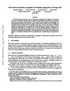
Figure 1: Graphical representation of a dynamic Bayesian network. general is that it does not always converge [25]. An important and open question is whether this is due to the graphical structure (e.g. messages running in cycles in networks with loops), to projections in the message update (causing interference between forward and backward passes even in chains), or both. By restricting ourselves to approximate inference on chains, we focus on the impact of the projections, unconcealed by structural effects. In an attempt to derive convergent algorithms, we first have to define what we would like to optimize. Inspired by the Bethe free energy recently proposed for loopy belief propagation [38] and its generalization to expectation propagation [24, 23], we derive in Section 4.1 a similar functional for expectation propagation in dynamic Bayesian networks. It is easy to show that fixed points of expectation propagation correspond to extrema of this free energy and vice versa. The primal objective boils down to a non-convex minimization problem with linear constraints. In Section 4.3 we turn this into a constrained convex minimization problem at the price of an extra minimization over canonical parameters. This formulation suggests a double-loop algorithm, which is worked out in Section 5. This double-loop algorithm is guaranteed to converge, but requires full completion of each inner loop. The equivalent description in terms of a saddle-point problem in Section 6 suggests faster short-cuts. The first one can be loosely interpreted as a combination of (natural) gradient descent and ascent. The second one is based on a damped version of “standard” expectation propagation. Both algorithms can be shown to be locally stable close to the saddle point. Simulation results regarding expectation propagation applied to switching linear dynamical systems are presented in Section 7. It is shown that it makes perfect sense to try and find the minimum of the free energy even when standard undamped expectation propagation does not converge. In Section 8 we end with conclusions and a discussion of implications for approximate inference in general Bayesian networks.
2
Dynamic Bayesian networks
2.1
Probabilistic description
We consider general dynamic Bayesian networks with latent variables xt and observations yt . The graphical model is visualized in Figure 1 for T = 4 time slices. The joint distribution of latent variables x1:T and observables y1:T can be written in the form P (x1:T , y1:T ) =
T Y
ψt (xt−1 , xt , yt ) ,
t=1
where ψt (xt−1 , xt , yt ) = P (xt |xt−1 )P (yt |xt ) , and with the convention ψ1 (x0 , x1 , y1 ) ≡ ψ1 (x1 , y1 ), i.e., P (x1 |x0 ) = P (x1 ), the prior. Our definition of the potentials ψt (xt−1 , xt , yt ) is sketched in Figure 2. In the following we will use the shorthand ψt (xt−1,t ) ≡ ψt (xt−1 , xt , yt ). That is, we will assume that all evidence y1:T is fixed and given and include the observations in the definition of the potentials. In principle, xt can be any combination of discrete and continuous variables (as for example in a switching linear dynamical systems). However, for notational convenience we will stick to integral notation. 3
x1
x1
/ x2
x2
/ x3
x3
/ x4
�
�
�
�
y1
y2
y3
y4
ψ1 (x1 ) = P (y1 |x1 )P (x1 )
ψ2 (x1 , x2 ) = P (y2 |x2 )P (x2 |x1 )
ψ3 (x2 , x3 ) = P (y3 |x3 )P (x3 |x2 )
ψ4 (x3 , x4 ) = P (y4 |x4 )P (x4 |x3 )
Figure 2: Definition of potentials. oo
α1 β1
/ x 1 o
α1
/
oo
β1
ψ1
α2 β2
/ x 2 o
α2
/
oo
β2
ψ2
α3
/ x 3 o
β3
ψ3
α3
/
oo
β3
α4
/ x 4
β4
ψ4
Figure 3: Message propagation.
2.2
Belief propagation
Our goal is to compute one-slice marginals or “beliefs” of the form P (xt |y1:T ): the probability of the latent variables in a given time slice given all evidence. This marginal is implicitly required in many EM-type learning procedures (e.g., the Baum-Welch procedure for hidden Markov models [3, 36] or parameter estimation in linear dynamical systems [34, 7]), but can also be of interest by itself, especially when the latent variables have a direct interpretation. Often we also need the two-slice marginals P (xt−1 , xt |y1:T ), but as we will see, belief propagation gives these more or less for free. A well-known procedure for computing beliefs in general Bayesian networks is Pearl’s belief propagation [29]. Specific examples of belief propagation applied to Bayesian networks are the forward-backward algorithm for hidden Markov models [31, 36] and the Kalman filtering and smoothing equations for linear dynamical systems [32, 7]. Here we will follow a description of belief propagation as a specific case of the sum-product rule in factor graphs [17]. This description is symmetric with respect to the forward and backward messages, contrary to the perhaps more standard filtering and smoothing operations. We distinguish variable nodes xt and local function nodes ψt in between variable nodes xt−1 and xt . The message from ψt forward to xt is called αt (xt ) and the message from ψt back to xt−1 is referred to as βt−1 (xt−1 ) (see Figure 3). The belief at variable node xt is the product of all messages sent from neighboring local function nodes: P (xt |y1:T ) ∝ αt (xt )βt (xt ) . Following the sum-product rule for factor graphs, the message sent from the variable node xt to the function node ψt is the product of all messages that xt receives, except the one from ψt itself. Or, to put it differently, the belief at xt divided by the message βt (xt ), which is (up to irrelevant normalization constants) αt (xt ). Note that this a peculiar property of chains: variable nodes simply pass the message they receive on to the next local function node; in a general tree-like structure these operations are slightly more complicated. Information about the potentials is incorporated at the corresponding local function nodes. The recipe for computing the message from the local function node ψt to a neighboring variable node xt′ , where t′ can be either t (forward message) or t − 1 (backward message), is as follows.1 1
The standard description is slightly different. In the first step the potential is multiplied with all messages excluding the message from xt′ to ψt and there is no division afterwards. For exact belief propagation, marginalization over all variables except xt′ commutes with the multiplication by the message from xt′ , which therefore
4
1. Multiply the potential corresponding to the local function node ψt with all messages from neighboring variable nodes to ψt , yielding Pˆ (xt−1 , xt ) ∝ αt−1 (xt−1 )ψt (xt−1,t )βt (xt ) ,
(t = 1 : T )
(1)
our current estimate of the distribution at the local function node given the incoming messages αt (xt−1 ) and βt (xt ). 2. Integrate out all variables except variable xt′ to obtain the current estimate of the one-slice marginal Pˆ (xt′ ). 3. Conditionalize, i.e., divide by the message from xt′ to ψt . Applying this recipe to the forward and backward messages we obtain, respectively, αt (xt ) ∝ =
βt−1 (xt−1 ) ∝ =
Z
dxt−1 αt−1 (xt−1 )ψt (xt−1 , xt )βt (xt )
Z
dxt−1 αt−1 (xt−1 )ψt (xt−1 , xt )
βt (xt ) (t = 1 : T )
Z
dxt αt−1 (xt−1 )ψt (xt−1 , xt )βt (xt )
Z
dxt ψt (xt−1 , xt )βt (xt ) ,
αt−1 (xt−1 ) (t = 2 : T )
(2)
with convention α0 (x0 ) ≡ βT (xT ) ≡ 1. It is easy to see that the forward and backward messages do not interfere: they can be computed in parallel and a single forward and backward pass is sufficient to compute the exact beliefs. Furthermore note that the two-slice marginals follow directly from (1) after all α1:T and β1:T have been calculated. Despite the apparent simplicity of the above expressions, even in chains exact inference can become intractable or computationally too expensive. We can think of the following, often related, causes for trouble. • The integrals at the function nodes are not analytically doable. This happens when, for example, the dynamics in the (continuous) latent variables is nonlinear. Popular approximate approaches are the extended Kalman filter [13] and recent improvements [15]. • The operations, i.e., the integrals or summations, at the function nodes become computationally too expensive because, for example, computing the integral involves operations that scale with a polynomial of the dimension of xt . This is the motivation behind variational approximations for factorial hidden Markov models [9], among others. Our own specific interest is in dynamic hierarchical models, the graphical structure of which is visualized in Figure 4. All nodes are Gaussian and all transitions linear, which makes this a specific case of a linear dynamical system. Exact inference is of order N 3 , with N the number of nodes within each time slice. The goal is to find an approximate inference algorithm that is linear in N . • A description of the belief states P (xt ) themselves is already exponentially large. For example, with N binary states at each time, we need on the order of 2N parameters to specify the probability P (xt ). The Boyen-Koller algorithm [4] projects the belief onto an approximate factored belief state that requires only N variables. The factored frontier algorithm [27] is a further extension that executes the forward and backward operations in a computationally efficient manner. cancels with the division afterwards [see Equation (2)]. This makes the standard procedure more efficient. The procedure outlined in the text is, as for as the results are concerned, equivalent and generalizes directly to the expectation propagation algorithm described in the next section.
5
m1
/ m2
/ m3
/ m4
�
� / z21
� / z31
� / z41
z11 �
�
�
�
y11
y21
y31
y41
� / z22
� / z32
� / z42
�
z12 �
�
�
�
y12
y22
y32
y42
� / z23
� / z33
� / z43
�
z13 �
�
�
�
y13
y23
y33
y43
Figure 4: A dynamic hierarchical model. s1
/ s2 / s3 / s4 BB BB BB BB BB BB BB BB BB BB � BB � BB � � ! ! ! / z2 / z3 / z4 z1 � �
� �
� �
� �
y1
y2
y3
y4
Figure 5: Switching linear dynamical system. • Over time, the number of components needed to describe the beliefs becomes exponential. This is the case in switching linear dynamical systems [35, 26] (see Figure 5). Suppose that we have M different switch states. Then, at each forward step the number of mixture components multiplies by M and we need M T mixture components to express the exact posterior. This is an example of the well-known fact that inference in hybrid Bayesian networks is much harder than in networks with just discrete or just Gaussian nodes [20]. Most of these problems can be tackled by the approach described below, which we will refer to as expectation propagation.
3
Expectation propagation as approximate belief propagation
3.1
Projection to the exponential family
Expectation propagation is a straightforward generalization of exact belief propagation. As explained above, problems with exact inference may arise in the marginalization step: exact calculation may not be doable and/or might not keep the beliefs within a family of distributions that is easy to describe and keep track of. The suggestion is therefore to work with approximate belief states, rather than with the exact ones. That is, we extend the marginalization step as follows. 2. Integrate out all variables except variable xt′ to obtain the current estimate of the belief state Pˆ (xt′ ) and project this belief state on to a chosen family of distribution, yielding the approximate belief qt′ (xt′ ). The remaining questions are then how to choose the family of distributions and how to project.
6
For the family of distributions we take a particular member of the exponential family, i.e., T
qt (xt ) ∝ eγt f (xt ) ,
(3)
(t = 1 : T )
with γ t the canonical parameters and f (xt ) the sufficient statistics.2 Typically, γ and f (x) are vectors with many components. For example, the sufficient statistics for an N -dimensional Gaussian are f (x) = {xi (i = 1 : N ), xi xj (i, j = 1 : N ; j ≤ i)} . Furthermore, note that a distribution over discrete variables can be written in exponential form, simply by defining f (x) as a long vector of Kronecker delta-functions, one for each possible state, and taking the corresponding component of γ equal to the logarithm of the probability of this state. Our choice for the exponential family is motivated by the fact that multiplication and division of two exponential forms yields another exponential form. That is, if we initialize the forward and backward messages as T
T
αt (xt ) ∝ eαt f (xt ) and βt (xt ) ∝ eβt f (xt ) , for example choosing αt = β t = 0, they will stay of this form: αt and β t fully specify the messages and are all that we have to keep track of. As in exact belief propagation, the belief qt (xt ) is a product of incoming messages: T f (x
qt (xt ) ∝ e(αt +βt )
t)
.
(4)
(t = 1 : T )
Typically, there are two kinds of reasons for making a particular choice within the exponential family. • The main problem is that the exact belief is not in the exponential family and therefore difficult to handle. The approximating distribution is of a particular exponential form, but usually further completely free. Examples are a Gaussian for the nonlinear Kalman filter or a conditional Gaussian for the switching Kalman filter of Figure 5. • The exact belief is in the exponential family, but requires too many variables to fully specify it. The approximate belief is part of the same exponential family but with additional constraints for simplifications, e.g., factorized over (groups of) variables. This is the case for the Boyen-Koller algorithm [5] and would also be the way to go for the linear dynamical system of Figure 4. Although the motivation is somewhat different, both can be treated within the same framework. In the projection step, we replace the current estimate Pˆ (x) by the approximate q(x) of the form (3) that is closest to Pˆ (x) in terms of the Kullback-Leibler divergence KL(Pˆ |q) =
Z
"
Pˆ (x) dx Pˆ (x) log q(x)
#
.
(5)
With q(x) in the exponential family, it is easy to show that the solution follows from moment matching: we have to find the canonical parameters γ such that g(γ) ≡ hf (x)iq ≡ 2
Z
dx q(x)f (x) =
Z
dx Pˆ (x)f (x) .
A perhaps more standard definition of a distribution in the exponential family reads q(x) = exp
" X
γi fi (x) + D(x) + S(γ)
i
#
,
which can be turned into the form (3) by defining f0 (x) ≡ D(x) and γ0 ≡ 1. The only thing to keep in mind then is that γ0 is never to be treated as a parameter, but always kept fixed.
7
For members of the exponential family the so-called link function g(γ) is unique and invertible, i.e., there is a one-to-one mapping from canonical parameters to moments. In fact, to compute new messages αt (xt ) and βt−1 (xt−1 ), we do not have to compute the approximate marginals Pˆ (xt′ ). We only need the expectation of f (xt′ ) over the two-slice marginal T
T
pˆt (xt−1,t ) ≡ Pˆ (xt−1 , xt ) ∝ eαt−1 f (xt−1 ) ψt (xt−1,t )eβt f (xt ) .
(t = 1 : T )
(6)
In terms of the canonical parameters αt and β t , the forward and backward passes require the following operations. Forward pass. Compute αt such that hf (xt )ipˆt = hf (xt )iqt = g(αt + β t ) .
(t = 1 : T )
Note that hf (xt )ipˆt only depends on the messages αt−1 and β t . With β t kept fixed, the ˜ t (αt−1 , β t ) can be computed by inverting g(·), i.e., translating from a solution αt = α moment form to a canonical form. Backward pass. Compute β t−1 such that hf (xt−1 )ipˆt = hf (xt−1 )iqt−1 = g(αt−1 + β t−1 ) .
(t = 2 : T )
˜ (αt−1 , β ). By Similar to the forward pass, the solution can be written β t−1 = β t−1 t definition we can set β T ≡ 0 (no information propagating back from beyond T ). The order in which the messages are updated is free to choose. However, iterating the standard forward-message passes seems to be most logical. 1. Start with all αt and β t equal to zero. 2. Go forward by updating α1 to αT leaving all β t intact. 3. Go backward by updating β T −1 to β 1 leaving all αt intact. 4. Iterate the forward and backward passes 2. and 3. until convergence. Note that we can set β T = 0 and can evaluate αT once after convergence: it does not affect the other αt and β t . Without projection, i.e., if the exponential distribution is not an approximation but exact, we have a standard forward-backward algorithm, guaranteed to converge in a single forward and ˜ t (αt−1 , β t ) = α ˜ t (αt−1 ), independent of β t backward pass. In these cases, one can easily show α ˜ (αt−1 , β ) = β ˜ (β ): the forward and backward messages do not interfere and similarly β t−1 t t−1 t and there is no need to iterate. This is the case for standard Kalman smoothing [32] and for the forward-backward algorithm for hidden Markov models [31]. Expectation propagation generalizes several known algorithms. For example, GPB2 for generalized pseudo-Bayes [2, 16], arguably the most popular inference algorithm for a switching linear dynamical system, is nothing but a single forward pass of the above algorithm. The BoyenKoller algorithm [5] corresponds to one forward and one backward pass for a dynamical Bayesian network with discrete nodes and independency assumptions over nodes within each time slice. In both cases, expectation propagation can be interpreted as an attempt to iteratively improve the existing estimates. Some of the problems mentioned in the previous section may not have been solved. For example, we may still have to compute complicated nonlinear or highly dimensional integrals or summations. However, in any case we “only” have to compute moments of the two-slice distribution, not the one-slice marginals themselves. A more important concern is that the exact beliefs might not be accurately approximated with a distribution in the exponential family. 8
ψt−1
ψt−2
exact posterior z
}|
{
z
}|
ψt+1
ψt {
z
}|
{
z
messages . . . β t−3 αt−2 β t−2 αt−1 β t−1 αt approximation
|
{z
}
qt−2
|
{z
qt−1
}
|
qt
ψt+2 {
z
}|
{
αt+1 β t+1 αt+2 . . .
βt {z
}|
}
|
{z
qt+1
}
Figure 6: Expectation propagation for dynamic Bayesian networks. The approximate distribution is a product of one-slice beliefs qt . Each belief qt follows from the product of the forward message αt and backward message β t . The product of the messages corresponding to β t−1 and αt represents the “effect” of potential ψt . That is, to recompute the effect of ψt , we take out the terms β t−1 and αt from the approximate distribution, substitute ψt instead, and project back to an uncoupled approximate distribution, yielding updates for qt−1 and qt and thus for β t−1 and αt .
3.2
Link with expectation propagation
Here we will illustrate that the algorithm described in the previous section is indeed a special case of expectation propagation as described in [25, 24]. We approximate the full posterior, which is a product of potentials or “terms” ψt (xt−1,t ), with an uncoupled distribution of exponential form: P (x1:T |y1:T ) ≈
T Y
qt (xt ) ∝
t=1
T Y
T f (x
e(αt +βt )
t)
.
t=1
Here αt and β t are supposed to quantify how adding a potential affects the approximate belief qt (xt ): αt stands for the effect of adding ψt (xt−1,t ), β t for the effect of adding ψt+1 (xt,t+1 ). Now suppose that we would like to recompute the effect of the potential ψt (xt−1,t ). We remove the corresponding terms αt and β t−1 and replace them with ψt (xt−1,t ) to arrive at the new approximation Pˆ (x1:T ) ∝
Y
t′ t
and thus at the approximate marginal over two time slices T 1 T Pˆ (xt−1 , xt ) ≡ pˆt (xt−1,t ) = eαt−1 f (xt−1 ) ψt (xt−1,t )eβt f (xt ) , ct
(t = 1 : T )
with ct a normalization constant and as above with convention Pˆ (x0 , x1 ) ≡ Pˆ (x1 ). These normalization constants can be used to estimate the data likelihood: P (y1:T ) ≈
T Y
ct .
t=1
3.3 3.3.1
Examples Switching linear dynamical system
Here we will illustrate the operations required for application of expectation propagation to switching linear dynamical systems. The potential corresponding to the switching linear dynamical system graphically visualized in Figure 5 can be written ψt (st−1 = i, st = j, zt−1 , zt ) = pψ (st = j|st−1 = i)Φ(zt ; Cij zt−1 , Rij )Φ(yt ; Aj zt , Qj ) , 9
where Φ(z; m, V ) stands for a Gaussian with mean m and covariance matrix V . The messages are taken to be conditional Gaussian potential of the form α αt−1 (st−1 = i, zt−1 ) ∝ pα (st−1 = i)Ψ(zt−1 ; mαi,t−1 , Vi,t−1 ) β βt (st = j, zt ) ∝ pβ (st = j)Ψ(zt ; mβj,t , Vj,t ),
where the potential Ψ(z; m, V ) is of the same form as Φ(z; m, V ), but without the normalization and in fact need not be normalizable, i.e., can have a negative covariance. Note that a message α(st−1 , zt−1 ) is in fact a combination of M Gaussian potentials, one for each switch state i. It can be written in exponential form with sufficient statistics f (s, z) = {δs,i (i = 1 : M ), δs,i zk (i = 1 : M ; k = 1 : N ), δs,i zk zl (i = 1 : M ; k, l = 1 : N ; l ≤ k)} . The two-slice marginal Pˆ (st−1 , st , zt−1 , zt ), with elements Pˆt (st−1 = i, st = j, zt−1 , zt ) ∝ αt−1 (st−1 = i, zt−1 )Φt (st−1 = i, st = j, zt−1 , zt )βt−1 (st = j, zt ) , consists of M 2 Gaussians: one for each combination {i, j}. With some bookkeeping, which involves the translation from canonical parameters to moments, we can compute the moments of these M 2 Gaussians, i.e., we can rewrite ˆ ij , Vˆij ) , Pˆ (st−1 = i, st = j, zt−1 , zt ) ∝ pˆij Φ(zt−1 , zt ; m
(7)
ˆ ij is a 2N -dimensional vector and Vˆij a 2N × 2N covariance matrix. where m To obtain the forward pass in expectation propagation, we have to integrate out zt−1 and sum over st−1 . Integrating out zt−1 is trivial: ˆ ij , Vˆij ) , Pˆ (st−1 = i, st = j, zt ) ∝ pˆij Φ(zt ; m ˆ ij and Vˆij are supposed to be restricted to the components corresponding to zt , i.e., where now m the components N + 1 to 2N in the means and covariances of (7). Summation over st−1 yields a mixture of M Gaussians for each switch state j, which is not a member of the exponential family. The conditional Gaussian of the form ˆ j , Vˆj ) qt (st = j, zt ) = pˆj Φ(zt |m closest in KL-divergence to this mixture of Gaussians follows from moment matching: pˆj =
X
ˆj = pˆij , m
i
and Vˆj =
X
ˆ ij , pˆij m
i
X i
pˆij Vˆij +
X
ˆ ij − m ˆ i )(m ˆ ij − m ˆ i )T . pˆij (m
i
To find the new forward message αt (st , zt ) we have to divide the approximate belief qt (st , zt ) by the backward message βt (st , zt ). This is most easily done by translating qt (st , zt ) from the moment form above to a canonical form and subtracting the canonical parameters corresponding to βt (st , zt ) to yield the new αt (st , zt ) in canonical form. The procedure for the backward pass follows in exactly the same manner by integrating out zt and summing over st . All together, it is just a matter of bookkeeping, with frequent transformations from canonical to moment form and vice versa. Efficient implementations can be made if, for example, the covariance matrices Qi and Ri are restricted to be diagonal. The forward filtering pass is equivalent to a method called GPB2 [2, 16]. An attempt has been made to obtain a similar smoothing procedure, but this required quite some additional approximations [26]. In the above description however, forward and backward passes are completely symmetric and smoothing does not require any additional approximations beyond the ones already made for filtering. Furthermore, the forward and backward passes can be iterated until convergence in the hope to find a more consistent and better approximation. 10
3.3.2
Dynamic hierarchical model
As a second example, we consider the dynamic hierarchical model of Figure 4. For ease of notation, we assume all nodes to correspond to one-dimensional variables zi,t and use z0,t to denote the highest-level node (referred to as mt in the figure). zt refers to the state of all hidden variables in time slice t. In this notation, the potentials are of the form ψt (zt−1,t ) =
N Y
P (yi,t |zi,t )P (zi,t |zi,t−1 , z0,t )P (z0,t |z0,t−1 ) .
i=1
We take the messages to be independent Gaussians, i.e., αt (zt ) =
N Y
αi,t (zi,t ) ,
i=0
with αi,t (xi,t ) one-dimensional Gaussians, and similarly for βt (zt ). All messages being independent, it is easy to see that the approximate two-slice marginal obeys Pˆ (zt−1,t ) = Pˆ (z0,t−1 , z0,t )
N Y
Pˆ (zi,t−1 , zi,t |z0,t ) ,
i=1
i.e., the distributions over the lower-level nodes are independent of each other given the higher level node. Straightforwardly collecting terms, we have Pˆ (zi,t−1 , zi,t |z0,t ) =
1 αi,t−1 (zi,t−1 )P (yi,t |zi,t )P (zi,t |zi,t−1 , z0,t )βi,t (zi,t ) , ci,t (z0,t )
(8)
with ci,t (z0,t ) the appropriate normalization constant and thus Pˆ (z0,t−1 , z0,t ) ∝ α0,t−1 (z0,t−1 )P (z0,t |z0,t−1 )β0,t (z0,t )
Y
ci,t (z0,t ) .
(9)
i
Note that these normalizations can be written in the form of a Gaussian potential and can be computed independently of each other. In the forward pass, we have to integrate out z0,t−1 in (9) yielding Pˆ (z0,t ). Similarly, we can integrate over zi,t−1 in (8) to obtain Pˆ (zi,t |z0,t ) and from that the approximate belief Pˆ (zi,t ) =
Z
dz0,t Pˆ (zi,t |z0,t )Pˆ (z0,t ) .
Again, the backward pass proceeds in a completely symmetric manner by integrating out z0,t and zi,t . The above scheme can be easily generalized to more than two levels. An update starts at the lowest level, conditioned on the parameters of the next level. Normalizing terms for the lower level then appear in the update for the next level. So we can go up to the highest level, always taken into account the normalization terms of the next lower level and conditioned on the parameters of the next higher level. The highest level is unconditioned and thus directly yields the required marginal distribution. The projection to a factorized form then goes in the opposite direction, subsequently integrating out over the distribution at the next higher level. The number of computations required in each forward and backward is proportional to the number of nodes (N + 1 in the above two-level case), to be contrasted with the N 3 complexity for exact inference. Obviously, exactly the same procedure can be used if all nodes are discrete rather than Gaussian.
11
4 4.1
A free energy function The free energy
In order to derive a convergent algorithm, we first have to define what we would like to optimize. The primal objective that we will derive is inspired by the recently proposed Bethe free energy functional for loopy belief propagation in [38] and follows the reasoning in [23]. The exact posterior P (x1:T |y1:T ) is the solution of P (x1:T |y1:T ) = argmin KL(Pˆ (x1:T )|P (x1:T |y1:T )) Pˆ (x1:T )
= argmin Pˆ (x1:T )
Z (
dx1:T
= argmin − Pˆ (x1:T )
"
Pˆ (x1:T )P (y1:T ) Pˆ (x1:T ) log P (x1:T , y1:T )
T Z X
dx1:T
#
Pˆ (x1:T ) log ψt (xt−1,t ) +
t=1
Z
dx1:T
)
Pˆ (x1:T ) log Pˆ (x1:T )
, (10)
under the constraint that Pˆ (x1:T ) is a probability distribution, i.e., is nonnegative and marginalizes to 1. Here and in the following this constraint is always implicitly assumed when we consider probability distributions and marginals. We will use notation min′ to indicate that there are other constraints as well (which ones should be clear from the text). The above expression is nothing but a definition of the conditional P (x1:T |y1:T ). In the following we will simplify and approximate it. The first observation is that the exact solution can be written as a product of two-slice marginals divided by a product of one-slice marginals:
Pˆ (x1:T ) =
T Y
Pˆ (xt−1,t )
t=1 TY −1
,
(11)
Pˆ (xt )
t=1
again with convention Pˆ (x0 , x1 ) ≡ Pˆ (x1 ). Plugging this into (10), our objective is to minimize min
Pˆ (x1:T )
(
T Z X t=1
"
#
)
TX −1 Z Pˆ (xt−1,t ) dxt−1,t Pˆ (xt−1,t ) log − dxt Pˆ (xt ) log Pˆ (xt ) ψt (xt−1,t ) t=1
,
for a distribution Pˆ (x1:T ) of the form (11). This can be rewritten as a minimization over two-slice marginals under consistency constraints Z
dxt−1 Pˆ (xt−1,t ) = Pˆ (xt )
(t = 1 : T )
and
Z
dxt Pˆ (xt−1,t ) = Pˆ (xt−1 )
(t = 2 : T )
.
(12)
We will refer to these as the forward and backward constraints, respectively. Note that there is no optimization with respect to beliefs P (xt ): these are fully determined given the two-slice marginals. For chains, and similarly for trees, this is all still exact. In networks containing loops, a factorization of the form (11) serves as an approximation (see e.g. [38]). The connection with variational approaches [14] is discussed in Section 8.
4.2
An approximate free energy
Now, in order to arrive at a free energy functional for expectation propagation we make two assumptions or approximations. First, we assume that the beliefs are of the exponential form P (xt ) ≈ qt (xt ) in (3). Next we replace the marginalization constraints (12) by weaker expectation constraints on pˆt (xt−1,t ) ≈ Pˆ (xt−1,t ): hf (xt )ipˆt = hf (xt )iqt
(t = 1 : T )
and hf (xt−1 )ipˆt = hf (xt−1 )iqt−1 12
(t = 2 : T )
.
(13)
Our objective remains the same, i.e., min
′
pˆ
(
T Z X t=1
"
#
TX −1 pˆt (xt−1,t ) dxt−1,t pˆt (xt−1,t ) log − ψt (xt−1,t ) t=1
Z
)
dxt qt (xt ) log qt (xt )
,
(14)
but now under the constraints (13) and with qt (xt ) of the exponential form (3). Note that, as before, these constraints make the one-slice marginals qt (xt ) an implicit function of the twoslice marginals pˆt (xt−1,t ): there is no minimization or maximization with respect to qt (xt ). Furthermore, qT (xT ) does not appear in the objective: it can be computed afterwards from the forward constraint (13) for t = T . Adding Lagrange multipliers β t and αt for the forward and backward constraints and taking derivatives we find that at a fixed point of (14) qt (xt ) and pˆt (xt−1,t ) are of the form (4) and (6). The other way around, at a fixed point of expectation propagation, the expectation constraints are automatically satisfied. Combination of these two observations proves that the fixed points of expectation propagation indeed correspond to fixed points of the “free energy” (14).
4.3
Bounding the free energy
Finding the minimum of the “primal” energy function (14) is a constrained optimization problem over functions. Due to the negative q log q term, this objective is not necessarily convex in pˆ1:T . To get rid of the concave q log q term, we make use of the Legendre transformation −
Z
�
dxt qt (xt ) log qt (xt ) = min −γ Tt hf (xt )iqt + log γt
Z
T
dxt eγt f (xt )
�
.
(15)
Substitution into (14) yields3 ′
min min γ pˆ
(
T Z X t=1
"
#
TX −1 pˆt (xt−1,t ) + −γ Tt hf (xt )iqt + log dxt−1,t pˆt (xt−1,t ) log ψt (xt−1,t ) t=1
�
Z
dxt e
γT t f (xt )
�)
.
(16) Now that we have eliminated the concave term, the remaining functional in (16) is convex in pˆ. The price that we had to pay is an extra minimization with respect to γ. An alternative and in fact equivalent interpretation of the Legendre transformation is the linear bound Z Z dxt qt (xt ) log qt (xt ) ≤ dxt qt (xt ) log qtold (xt ) ,
where qtold (xt ) can be any distribution and is typically the solution given the old parameter settings (here the two-slice marginals pˆt (xt−1,t ) and pˆt+1 (xt,t+1 )). In the following we will stick to the explicit minimization over γ to make the connection with expectation propagation below. Both formulations suggest a double-loop algorithm: in the inner loop we keep γ fixed and minimize with respect to pˆ under the appropriate constraints; in the outer loop we keep pˆ fixed and minimize with respect to γ.
5
A convergent algorithm
5.1
The inner loop
Let us first focus on the inner loop for fixed γ. We are left with a convex minimization problem with linear constraints, which can be turned into a dual unconstrained concave maximization problem in terms of Lagrange multipliers (see e.g. [21]). 3
For ease of notation, γ and pˆ without subscript refer to all relevant γ t and pˆt (here γ 1:T −1 , often γ 1:T ).
13
5.1.1
The dual objective
To get rid of any dependency on qt (xt ), we substitute the constraint4 hf (xt )iqt =
i 1h hf (xt )ipˆt + hf (xt )ipˆt+1 2
(t = 1 : T − 1)
in (16) and neglect terms independent of pˆt to arrive at the objective min pˆ
′
( T Z X t=1
"
)
#
−1 h i pˆt (xt−1,t ) 1 TX dxt−1,t pˆt (xt−1,t ) log γ Tt hf (xt )ipˆt + hf (xt )ipˆt+1 − ψt (xt−1,t ) 2 t=1
.
(17)
The only remaining constraints are now “forward equals backward”, i.e., hf (xt )ipˆt = hf (xt )ipˆt+1 .
(t = 1 : T − 1)
Introducing Lagrange multipliers δ t /2 and collecting all terms in the Lagrangian that depend on pˆt (xt−1,t ), we obtain Z
(
)
#
"
1 1 pˆt (xt−1,t ) − (γ t − δ t )T f (xt ) − (γ t−1 + δ t−1 )T f (xt−1 ) dxt−1,t pˆt (xt−1,t ) log ψt (xt−1,t ) 2 2
,
(t = 1 : T )
(18) where we have the convention that γ 0 ≡ δ 0 ≡ γ T ≡ δ T ≡ 0. Taking the functional derivative with respect to pˆt (xt−1,t ) we regain the form (6) if we substitute 1 1 αt−1 = (γ t−1 + δ t−1 ) and β t = (γ t − δ t ) . 2 2
(19)
(t = 1 : T )
Substitution into the Lagrangian (18) and back into (17) yields the dual objective max F1 (δ) where F1 (δ) = − δ
T X t=1
log
Z
1
T f (x
dxt−1,t e 2 (γt−1 +δt−1 )
t−1 )
1
T f (x
ψt (xt−1,t )e 2 (γt −δt )
t)
.
(20) Again recall that qT (xT ) does not appear in the primal objective, and there is no optimization with respect to δ T in the dual objective. We can always compute the approximate belief qT (xT ) afterwards from pˆT (xT −1,T ). 5.1.2
Unconstrained maximization
With the primal (17) being convex in pˆ, the dual F1 (δ) is concave in δ, and thus has a unique solution. In principle, any optimization algorithm will do, but here we will propose a specific one, which can be interpreted as a damped version of fixed-point iteration. ˜ ≡ ˜t ≡ α ˜ t (αt−1 , β t ) and β In terms of the standard forward and backward updates α t ˜ (αt , β ), with αt and β related to δ t and γ as in (19), the gradient with respect to β t t+1 t t δ t reads i 1h ∂F (δ) ˜ ) . ˜ t + β t ) − g(αt + β = g(α (21) t ∂δ t 2 Setting the gradient to zero suggests the update ˜ . ˜t − β δ new = δ˜t ≡ α t t
(22)
˜ =β ˜ (β ), this fixed point iteration ˜t = α ˜ t (αt−1 ) and β Without any projections, i.e., with α t t t+1 can be interpreted as finding the maximum of F (δ) in the direction of δ t , keeping the other 4 Any other convex linear combination of forward and backward expectations will do as well, but this symmetric choice appears to be most natural.
14
δ t′ fixed. Each update (22) would guarantee an increase of F (δ), unless the corresponding gradient (21) vanishes. ˜ do depend on δt (through αt and β , ˜ t and β However, in expectation propagation both α t t respectively) and the full update (22) does not necessarily go uphill. A simple suggestion is to consider a damped version of the form δ new = δ t + ǫδ (δ˜t − δ t ) . t
(23)
It is easy to show5 that this update is “aligned” with the gradient (21) and thus, with sufficiently small ǫδ , will always lead to an increase in F1 (δ). Expecting the dependency of δ˜t on δ t to be rather small, the hope is that we can take a rather large ǫδ . In terms of the moments, the update (23) reads h
�
�
�
δ new = δ t + ǫδ g−1 hf (xt )ipˆt − g−1 hf (xt )ipˆt+1 t
�i
,
(24)
i.e., to update a single δ t we have to compute one forward and one backward moment.
5.2
The outer loop
As could have been expected, especially in the interpretation of the Legendre transformation as a bounding technique, the outer loop is really straightforward. Setting the gradient of (16) with respect to γt (xt ) to zero yields the update g(γ new ) = hf (xt )iqt = t
i 1h hf (xt )ipˆt + hf (xt )ipˆt+1 , 2
(t = 1 : T − 1)
(25)
with pˆ the solution of the inner loop. In terms of the messages αt and β t and their standard ˜ this is equivalent to ˜ t and β expectation propagation updates α t γ new t
=g
−1
i�
� h 1
2
˜ ) + g(α ˜ t + βt ) g(αt + β t
.
(26)
With αt and β t the result of the maximization in the inner loop, we have δ t = δ˜t and thus ˜ =α ˜ t + β t . This can be used to simplify the update (26) to αt + β t γ new = γt + t
5.3
i 1h ˜ −γ . ˜t + β α t t 2
(27)
Link with Yuille’s CCCP
In [39], Yuille proposes a double-loop algorithm for (loopy) belief propatation and Kikuchi approximations. We will show the link with the above double-loop algorithm by describing what Yuille’s CCCP amounts to when applied to approximate inference in dynamic Bayesian networks. We rewrite the primal objective (14) as min pˆ
′
(
T Z X t=1
"
#
TX −1 pˆt (xt−1,t ) dxt−1,t pˆt (xt−1,t ) log +κ ψt (xt−1,t ) t=1
−(1 + κ)
TX −1 Z
)
dxt qt (xt ) log qt (xt )
t=1
Z
dxt qt (xt ) log qt (xt )
,
5 ˜ , the update (23) is proportional to δ˜ t − δ t = γ − γ and we can ˜ t + β t and γ 2 ≡ αt + β In terms of γ 1 ≡ α t 2 1 write ∂F (δ) = (γ 2 − γ 1 )T [g(γ 2 ) − g(γ 1 )] = KL(q1 |q2 ) + KL(q2 |q1 ) ≥ 0 , 2(δ˜ t − δ t )T ∂δ t with q1 and q2 the exponential distributions with canonical parameters γ 1 and γ 2 and link function g(·).
15
where κ can be any positive number (Yuille takes κ = 1). Now we apply the Legendre transformation (15) only to the second (negative) term to arrive at [compare with (16)] min min γ pˆ,q
(
′
T Z X t=1
"
#
TX −1 pˆt (xt−1,t ) dxt−1,t pˆt (xt−1,t ) log +κ ψt (xt−1,t ) t=1
+(1 + κ)
TX −1 �
−γ Tt
Z
hf (xt )iqt + log
t=1
γT t f (xt )
dxt e
Z
dxt qt (xt ) log qt (xt )−
�)
.
(28)
For convenience, we treat the one-slice marginals q as free parameters. Yuille’s CCCP algorithm is now nothing but an iterative minimization procedure on the objective (28). In the inner loop, we keep γ fixed and try and find the minimum with respect to pˆ and q under the constraints (13). Since the objective is convex in pˆ and q for fixed γ, we can turn this into an unconstrained maximization problem over Lagrange multipliers. Introducing Lagrange multipliers γ − β and γ − α for the forward and backward constraints, respectively, and minimizing with respect to pˆt and qt , we obtain qt (xt ) ∝ eγˆ t ft (xt ) T f (x
pˆt (xt−1,t ) ∝ e(γt−1 −βt−1 )
t−1 )
T f (x
ψt (xt−1,t )e(γt −αt )
t)
.
(t = 1 : T )
,
with
1 [γ − (αt + β t )] . κ t Substitution into (28) yields for the inner loop ˆ t ≡ γt − γ
(
max −κ α,β
TX −1 t=1
log
Z
dxt e
ˆT γ t f (xt )
−
T X t=1
log
Z
(γt−1 −βt−1 )T f (xt−1 )
dxt−1,t e
ψt (xt−1,t )e
(γt −αt )T f (xt )
)
.
(29) In the limit κ → 0, we regain the inner loop described in Section 5.1: the first term induces the constraint αt + β t = γ t , which we could get rid of by introducing δ t ≡ αt − β t . In Yuille’s CCCP inner loop the maximization is unconstrained. The extra q log q term complicates the analysis, but with the introduction of extra Lagrange multipliers for the normalization of pˆ and q, similar fixed point iterations can be found, at least in the situation without projections (as for loopy belief propagation). In any case, the unique solution of (29) obeys ˜t + αt = α
i h i 1 h ˜ ) and β = β ˜ + 1 ˜ ) , ˜t + β ˜ γ t − (α γ − ( α + β t t t t t 2+κ 2+κ t
(30)
which corresponds to our δ t = δ˜t with an additional change in αt + β t . This latter change vanishes in the limit κ → 0. The outer loop in Yuille’s CCCP algorithm minimizes (28) with respect to γ, keeping q fixed, and yields, after some manipulations using (30), ˆt = γt + γ new =γ t
i 1 h ˜ −γ , ˜t + β α t t 2+κ
(31)
to be compared with (27). Summarizing, the crucial trick to turn the constrained minimization of the primal, which consists of a convex and concave part, into something doable, is to get rid of the concave part through a Legendre transformation (or an equivalent bounding technique). The remaining functional in the two-slice marginals pˆ is then convex and can be “dualized”, yielding a maximization with respect to the Lagrange multipliers. Taking over part of the concave term to the convex side is unnecessary and makes the bound introduced through the Legendre transformation less accurate, yielding a (slightly and unnecessarily) less efficient algorithm. 16
6
Faster alternatives
6.1
Saddle-point problem
Explicitly writing out the constrained minimization in the inner loop into maximization over Lagrange multipliers δ, we can turn the minimization in (16) into the equivalent saddle-point problem min max F (γ, δ) with F (γ, δ) ≡ F0 (γ) + F1 (γ, δ) , γ
δ
where F0 (γ) =
TX −1
log
t=1
Z
T
dxt eγt f (xt ) ,
and where F1 (γ, δ) follows from (20) if we take into account its dependency on γ as well. Note that F (γ, δ) is concave in δ, but, through the dependency of F1 (γ, δ) on γ, non-convex in γ. We can guarantee convergence to a correct saddle-point with a double-loop algorithm that completes the concave maximization procedure in the inner loop before making the next step going downhill in the outer loop. This is, of course, exactly the procedure described in Section 5. The full completion of the inner loop seems quite inconvenient and a straightforward simplification is then to intermix updates in the inner and the outer loop. The first alternative that we will consider can be interpreted as a kind of natural gradient descent in γ and ascent in δ: decrease with respect to γ and increase with respect to δ can be guaranteed at each step, but this can, alas, not guarantee convergence to the correct saddle point. The second alternative is a damped version of “standard” expectation propagation as outlined in Section 3. In a first-order expansion around a saddle-point, both algorithms will be shown to be equivalent.
6.2
Combined gradient descent and ascent
Our first proposal is to apply the inner loop updates (24) in δ and outer loop updates (25) in γ sequentially. With each update, we can guarantee F (γ new , δ) ≤ F (γ, δ) ≤ F (γ, δ new ) ,
(32)
where to satisfy the second inequality, we may have to resort to a damped update in δ with ǫδ < 1. Note that the update (25) minimizes the primal objective with respect to γ t for any qt (xt ), not necessarily one that results from the optimization in the inner loop. However, the perhaps simpler update (27) is specific to δ being at a maximum of F1 (γ, δ) and cannot guarantee a decrease in F (γ, δ) for general δ.6 Alternatively, we can update δ t and γ t at the same time, for example damping the update in γ t as well, e.g. taking �
γ new = γ t + ǫγ g−1 t 6
� h 1
2
hf (xt )ipˆt + hf (xt )ipˆt+1
i�
− γt
�
In fact, even a damped version does not work. If it did, we should be able to show that the update in γ t is always in the direction of the gradient ∂γ t F (γ, δ), which boils down to (2γ 0 − γ 1 − γ 2 )T [2g(γ 0 ) − g(γ 1 ) − g(γ 2 )] ≥ 0 for all γ 0 , γ 1 , and γ 2 . This inequality is valid everywhere if and only if g(γ) is linear in γ. Otherwise we can construct cases that violate the inequality. For example, take γ1 = γ0 + ǫ1 and γ2 = γ0 − ǫ2 with ǫ1 and ǫ2 small and expand up to second order to get (in one-dimensional notation) (2γ0 − γ1 − γ2 ) [2g(γ0 ) − g(γ1 ) − g(γ2 )] = 4g ′ (γ0 )(ǫ1 − ǫ2 )2 + g ′′ (γ0 )(ǫ21 + ǫ22 )(ǫ1 − ǫ2 ) . Now we can always construct a situation in which the second term dominates the first (ǫ21 + ǫ22 ≫ ǫ1 − ǫ2 ≈ 0) and choose ǫ1 − ǫ2 such that this dominating term is negative. Such a situation is perhaps unlikely to occur in practice, but it shows that a downhill step cannot be guaranteed, not even for ǫγ small.
17
h
�
�
�
δ new = δ t + ǫδ g−1 hf (xt )ipˆt − g−1 hf (xt )ipˆt+1 t
�i
.
(33)
We can either update the canonical parameters for all t at the same time or one after the other, e.g., by going forward and backward as one would do in standard message passing. Both update schemes can be loosely interpreted as doing combined gradient descent in γ and gradient ascent in δ. Gradient descent-ascent is a standard approach in the field of optimization for finding saddle points of an objective function. Convergence to an, in fact unique, saddle point can be guaranteed if F (γ, δ) is convex in γ for δ and concave in δ for all γ, provided that the step sizes ǫδ and ǫγ are sufficiently small [30]. In our more general case, where F (γ, δ) need not be convex in γ for all δ, gradient descent-ascent may not be a reliable way of finding a saddle point. For example, it is possible to construct situations in which gradient descent-ascent leads to a limit cycle [33]. The most we can therefore say is that the above update schemes with sufficient damping are locally stable, i.e., will converge back to the saddle point if slightly perturbed away from it, if the functional F (γ, δ) is locally convex-concave.7 A more detailed proof for the updates (33) is given in the Appendix.
6.3
Damped expectation propagation
The joint updates (33) have the flavor of a damped update in the direction of “standard” expectation propagation, but are not exactly the same. Straightforwardly damping the full ˜ =β ˜ (αt , β ), we get ˜t = α ˜ t (αt−1 , β t ) and β new =α =β updates αnew t t t+1 t t ˜ t − αt ) αnew = αt + ǫ(α t new ˜ β = β t + ǫ(β t − β t ) ,
(34)
γ new = γ t + ǫ(˜ γ t − γt) t new ˜ δ = δ t + ǫ(δ t − δ t ) ,
(35)
t
or, in terms of γ and δ,
t
˜ . ˜t ≡ α ˜t + β with γ t This update for δ t is the same as in (33) if we take ǫδ = ǫ. The updates for γ t are slightly different. The connection between them becomes clearer when we take ǫγ = 2ǫ and rewrite (33) as ˜ t − γ t) , γ new = γ t + ǫ(∆t + γ t with ∆t ≡ 2g−1
� h 1
2
i�
˜ ) + g(α ˜ t + βt) g(αt + β t
�
�
˜ ] + [α ˜ t + βt ] . − [αt + β t
This term ∆t is then the only difference between the gradient descent-ascent updates (33) and the damped expectation propagation updates (35). Recall that it is zero at a particular maximum δ ∗ (γ), but not in general for all δ. However, local stability only depends on properties of the linearized versions of the updated close to the saddle point. In the Appendix it is shown that these coincide for the gradient descent-ascent and damped expectation propagation updates. Basically, both ∆t and its derivatives with respect to γ and δ vanish at a fixed point. Therefore, we can conclude that the damped expectation propagation updates (35) and (34) have the same local stability properties. Furthermore, since the ordering of updates does not affect these notions of stability in the limit of small ǫ, this also applies to a standard sequential message passing scheme. 7
While turning this report into a submission, we extended this argumentation and managed to prove the stronger statement that a stable fixed point of damped expectation propagation must correspond to a minimum of the Bethe free energy (but not necessarily the other way around). See the conference paper [12].
18
7
Simulation results
We have tested our algorithms on randomly generated switching linear dynamical systems. The structure of a switching linear dynamical system is visualized in Figure 5 and Section 3.3.1 describes “standard” expectation propagation propagation. We generated many random instances. Each instance is a combination of a switching linear dynamical system, consisting of all parameters specifying the model (observation and transition matrices, covariance matrices, and priors) and evidence y1:T . Each instance then corresponds to a particular setting of the potentials ψt (xt−1 , xt ). We generated all model parameters randomly and independently from “normal” distributions (e.g., elements of the observation matrices from a Gaussian with mean zero and unit variance, covariance matrices of order one from Wishart distributions, rows of the transition matrices between switches and continuous latent variables independently, and so on). We varied the length of the time sequence between 3 and 5, the number of switches between 2 and 4, and the dimension of the continuous latent variables and the observations between 2 and 4. The evidence that we used was generated by a switching linear dynamical system with the same “structure” (length of time sequence, number of switches, and dimensions), but different model parameters. In the following we will focus on the quality of the approximated beliefs Pˆ (xt |y1:T ) and compare them with the exact beliefs that result from the algorithm of [18] based on strong marginalP ization. As a quality measure we consider the Kullback-Leibler divergence KL ≡ Tt=1 KL(Pt |Pˆt ) between the exact beliefs Pt (xt ) and the approximate beliefs Pˆt (xt ), both of which are conditional Gaussians. Although any particular choice is somewhat arbitrary and depends on the application at hand, for the problems considered here (relatively small time sequences) we tend to make the following crude characterization. 101 100 10−2
KL > 101 > KL > 100 > KL > 10−2 > KL
useless doubtful useful excellent
In most cases (more than 95% of all instances generated following the procedure described above), “standard” (undamped) expectation propagation works fine and converges within a couple of iterations. For a typical instance (see Figure 7 on the left), the Kullback-Leibler divergence drops after a single forward pass (equivalent to GPB2, the standard procedure for inference in switching linear dynamical systems) to an acceptably low value, decreases a little more in the smoothing step, and perhaps a little further in one or two more sweeps until no more significant changes can be seen. Damped expectation propagation and the double-loop algorithm converge to the same fixed point, but are less efficient. The instances for which undamped expectation propagation does not converge can be roughly subdivided into two categories. The first category consists of instances that run into numerical problems, in some cases already in the forward pass. Damping as well as the double-loop algorithm seem to help in some cases, but in the end often also run into trouble when getting close to the fixed point. Instability is a well-known problem for inference in hybrid networks. It can occur especially when covariance matrices corresponding to the conditional probabilities of the continuous latent variables become singular. Solving this is an important subject, see e.g. [19], but beyond the scope of the current study. We therefore focus on the second category, where undamped expectation propagation gets stuck in a limit cycle. A typical instance is shown in Figure 7 on the right. Here the period of the limit cycle is 8 (eight sweeps, each consisting of a forward pass and a backward pass); smaller and even larger periods can be found as well. The approximate beliefs jump between 16 different solutions, ranging from “useful” to “useless”. Damping the belief updates a little, say with ǫ = 0.5 as in Figure 7, is for almost all instances sufficient to converge to a stable solution. Occasionally, in less than 1% of all “cyclical” instances 19
0
typical "easy" instance
typical "difficult" instance
2
10
10
KL−divergence
KL−divergence
−2
10
−4
10
−6
1
10
0
10
10
−8
10
0.5
−1
1 1.5 number of iterations
10
2
0
5
10 15 20 number of iterations
25
Figure 7: Typical examples of “easy” (left) and “difficult” (right) problems. Both are randomly generated instances of a switching linear dynamical systems with 3 switch states, 3-dimensional continuous latent variables, 4-dimensional observations, and sequence length T = 5. The KLdivergence between exact and approximated beliefs is plotted as a function of the number of iterations. Each iteration consists of a forward and a backward pass of expectation propagation. For the “easy” instance, nondamped expectation belief propagation converges in a few iterations. Without damping (solid line), the “difficult” instance gets stuck in a limit cycle of period 8. Damping with step size ǫ = 0.5 (dashed line) is sufficient to convergence to a stable fixed point. that we encountered, we did not manage to damp expectation propagation to a stable solution with reasonable values of the step size ǫ. An example is given in Figure 8. Lowering the step size ǫ mainly affects the period of the cycle, hardly its amplitude. The double-loop algorithm converges in several iterations (comparable to the number of iterations required for other instances) to a stable fixed point, which, in this case, happens to be rather far from the exact beliefs. A simple check reveals that this fixed point, by construction of the double-loop algorithm a local minimum of the free energy, is unstable under damped expectation propagation with step size as low as ǫ = 0.018 . In the recent literature, it has been suggested at several places (see e.g. [37, 23]) that when undamped (loopy) belief propagation does not converge, it makes no sense to search for the minimum of the Bethe free energy with a more complicated algorithm: the failure of undamped belief propagation to converge indicates that the solution is inaccurate anyways. To check this hypothesis, we did the following experiment. For each of the 138 nonconvergent cyclic instances that we found, we generated another converging instance with the same “structure” (length of time sequence, number of switch states, and dimensions). As before, we refer to the former set of nonconvergent instances as “difficult” and the latter set of convergent instances as “easy”. In Figure 9 we have plotted the KL-divergences after a single forward pass (corresponding to GPB2) and after convergence (with damped expectation propagation or the double-loop algorithm for the difficult instances). Two important conclusions can be drawn. • It makes sense to search for the minimum of the free energy. For almost all instances, the beliefs corresponding to the minimum of the free energy are closer to the exact beliefs than the ones obtained after a single forward pass. This is not only the case for all 138 “easy” instances that we have seen, but also for almost all (132 out of 138) “difficult” ones. Given our crude subdivision between “useful” and “useless” or “doubtful” approximations based on the value of the KL-divergence (KL 1), the improvement can be considered relevant for many instances: for 64 out of 138 “easy” instances and for even 92 out of 138 8
See [12] for a possible explanation of this effect.
20
no damping
damping with step size 0.5
2
10
KL−divergence
KL−divergence
2
10
0
10
−2
10
1
10
0
10
−1
0
5
10 15 20 number of iterations
10
25
0
damping with step size 0.1
2
20
40 60 80 number of iterations
100
double−loop algorithm
KL−divergence
KL−divergence
10
1
10
0
10
−1
10
0
10
−1
0
100
200 300 400 number of iterations
10
500
0
10 20 number of iterations
30
Figure 8: A rare instance in which damping with reasonable values of the step size ǫ does not lead to convergence to a stable fixed point. Changing the step size ǫ from 1 (upper left: no damping) to 0.5 (upper right) and further to 0.1 (lower left) lengthened the period of the cycle, but (going from 0.5 to 0.1) hardly its amplitude. The double-loop algorithm (lower right) converges within a few iterations (each iteration consists of a full inner-loop maximization and outer-loop step). The KL-divergence corresponding to the minimum of the free energy obtained with the doubleloop algorithm is indicated with a dashed line in all plots for reference. This particular instance has 2 switch states, 3-dimensional continuous latent variables and observations, and T = 3.
21
"difficult" instances "easy" instances
KL after convergence
101
100
10−2
10−6 −2
10
−1
10
0
1
10
10
2
10
KL after forward pass Figure 9: KL-divergences for “easy” (‘o’, converging without damping) and “difficult” (‘+’, getting stuck in a limit cycle without damping) instances after a single forward pass of expectation propagation versus after convergence to a minimum of the free energy. The dashed line corresponds to no improvement (y = x). The dotted grid lines crudely subdivide the KL-divergences between more and less “useful” (KL smaller than or larger than 1, which is obviously somewhat arbitrary). It can be seen that searching for the minimum in almost all instances leads to an improvement in the accuracy of the approximate beliefs, often making the difference between more or less “useful” (all instances in the lower right corner). The histograms visualize the distributions of the KL-divergences along the corresponding axes (dashed for “easy” instances, solid for “difficult” ones). The overlap between both distributions indicates that (non-)convergence of undamped expectation propagation is not a clear-cut indicator for the applicability of the minimum of the free energy for approximate inference.
22
“difficult” instances. • Convergence of undamped belief propagation is not a clear-cut criterion for the quality of the approximation. Although the “easy” instances typically have a smaller KL-divergence than the “difficult” ones, there is considerable overlap both for the KL-divergence after a single forward pass and after convergence. For example, in 8 of the 138 cases the “difficult” instance happened to converge to a better (lower KL-divergence) solution than the corresponding “easy” one.
8
Discussion and conclusions
We have derived expectation propagation as a straightforward extension of exact belief propagation. The following ingredients are crucial to this simple interpretation. 1. A description of belief propagation that is symmetric with respect to the forward and backward messages. 2. The notion that we should better project the beliefs and derive the messages from these approximate beliefs, rather than approximating the messages themselves. The symmetric description dramatically simplifies smoothing in switching linear dynamical systems. In [26] an attempt has been made to derive an approximate smoothing procedure based on the asymmetric description of belief propagation in terms of filtered and smoothed estimates. The derivation of this procedure requires quite some additional assumptions, making it rather complicated and resulting in a highly specific implementation. The symmetric algorithm outlined in Section 3.3.1 is easy to implement and mainly boils down to the computation of the moments of a mixture of Gaussians, transformation of moment to canonical form and vice versa, and simple subtractions and additions of canonical parameters. Generalization of this procedure to message propagation in singly-connected or even loopy networks is straightforward. Applied to these networks, it would improve the “weak marginalization approach” outlined in [18]. Approximating the messages rather than the beliefs is tempting, especially when the messages themselves have a direct interpretation (e.g., αt (xt ) being proportional to the filtered estimate P (xt |y1:t ) and βt (xt ) to P (xt |yt+1:T )). Both are equivalent when the messages in the opposite direction are still the initial ones (i.e., set to 1), but can yield quite different approximate beliefs otherwise. Furthermore, when we approximate the beliefs, the forward and backward passes start to interfere, suggesting iterations as an attempt to improve our estimates. An iterative variant of the Boyen-Koller algorithm [5] has been applied in [27] with clear improvements. An important difference between greedy projection methods and variational approaches as in [14, 9, 8] is that the latter minimize a clearly and globally defined Kullback-Leibler divergence. A disadvantage of the variational approaches is that they minimize the Kullback-Leibler divergence with the approximate distribution Q and exact distribution P in the “wrong order”, i.e., they minimize KL(Q|P ), where minimizing KL(P |Q) seems to make better sense. Expectation propagation minimizes the “right” KL-divergence, as can be seen in (5), but does this in a greedy and local manner. The relationship between the variational approach and expectation propagation can be clarified in two different ways. • The Kullback-Leibler divergence corresponding to the variational approach is obtained if we substitute the two-slice marginal in the free energy (14) by the product of corresponding one-slice marginals, i.e., pˆt (xt−1,t ) = qt (xt−1 )qt (xt ) ,
23
and take the minimum with respect to the one-slice marginals qt of the chosen exponential form: min q1:T
′
(
XZ t
"
#
X qt−1 (xt−1 )qt (xt ) dxt−1,t qt−1 (xt−1 )qt (xt ) log − ψt (xt−1,t ) t
= min KL(Q|P ) with Q(x1:T ) = Q
Y
Z
)
dxt qt (xt ) log qt (xt )
qt (xt ) and P (x1:T ) ∝
Y
ψt (xt−1,t ) . (36)
t
t
• An equivalent definition of step 2 in expectation propagation (beginning of Section 3) is as follows. 2. Project the two-slice marginal Pˆ (xt−1,t ) on to the distribution qt−1 (xt−1 )qt (xt ), by minimizing the KL-divergence KL(Pˆt−1,t |qt−1 qt ) =
Z
dxt−1,t Pˆ (xt−1,t ) log
"
Pˆ (xt−1,t ) qt−1 (xt−1 )qt (xt )
#
,
(37)
with respect to qt′ (xt′ ) (keeping the other approximate belief fixed). This yields exactly the same procedure since integrating out all variables except xt′ , as in the original formulation, is then implicitly done while matching the moments. The variational approach can be obtained when we reverse the role of Pˆ (xt−1,t ) and qt−1 (xt−1 )qt (xt ) in the above KL-divergence.9 In much the same way as loopy belief propagation is an improvement over mean-field approximations [38], we expect expectation propagation to outperform a variational approach that is based on the same approximate structure (independent time slices in the above case of dynamic Bayesian networks). Some evidence for that can be found in [8], where the variational approach did not lead to better results than generalized pseudo-Bayes, which is just a single forward pass of expectation propagation. An important question is how the results obtained for chains in this article generalize to tree-like or even loopy structures. Analyzing loopy belief propagation (no projections, but a network structure containing loops) along the same lines, we arrive at a quite similar double-loop algorithm for guaranteed convergence and single-loop short-cuts [11]. Our current interpretation is that, as soon as messages start to interfere, which happens both with approximations and with loops but not with exact inference on trees, we have to take special care that we update the messages in a special way: going uphill relative to each other to satisfy the constraints, going downhill together to minimize the free energy. That damped versions of expectation propagation and loopy belief propagation seem to move in the right uphill/downhill directions might explain why single-loop algorithms converge well in many practical cases.
References [1] S. Amari. Natural gradient works efficiently in learning. Neural Computation, 10:251–276, 1998. 9
To see this, define qt (xt ) = αt (xt )βt (xt ) ,
and replace the minimization over q1:T in (36) by a joint minimization over α1:T and β1:T under the constraint that their product normalizes to 1 (and that both are of the chosen exponential form). Now consider the minimization of KL(P |Q) with respect to αt keeping all other α’s and β’s fixed. Collecting relevant and neglecting irrelevant terms, it is easy to see that min′ KL(Q|P ) = min′ KL(qt−1 qt |Pˆt−1,t ) , αt
αt
the KL-divergence of (37) in reverse order. In other words, greedy projection based on KL(qt−1 qt |Pˆt−1,t ) corresponds to some kind of iterative procedure for minimizing KL(Q|P ).
24
[2] Y. Bar-Shalom and X. Li. Estimation and Tracking: Principles, Techniques, and Software. Artech House, 1993. [3] L. Baum, T. Petrie, G. Soules, and N. Weiss. A maximization technique occurring in the statistical analysis of probabilistic functions of Markov chains. Annals of Mathematical Statistics, 41(1):164–171, 1970. [4] X. Boyen and D. Koller. Tractable inference for complex stochastic processes. In Proceedings of the Fourteenth Conference on Uncertainty in Artificial Intelligence, pages 33–42, San Francisco, 1998. Morgan Kaufmann. [5] X. Boyen and D. Koller. Approximate learning of dynamic models. In M. Kearns, S. Solla, and D. Cohn, editors, Advances in Neural Information Processing Systems 11, pages 396– 402. MIT Press, 1999. [6] A. Doucet, N. de Freitas, and N. Gordon, editors. Sequential Monte Carlo Methods in Practice, New York, 2001. Springer-Verlag. [7] Z. Ghahramani and G. Hinton. Parameter estimation for linear dynamical systems. Technical report, Department of Computer Science, University of Toronto, 1996. [8] Z. Ghahramani and G. Hinton. Variational learning for switching state-space models. Neural Computation, 12:963–996, 1998. [9] Z. Ghahramani and M. Jordan. Factorial hidden Markov models. Machine Learning, 29:245–275, 1997. [10] T. Heskes. On “natural” learning and pruning in multilayered perceptrons. Neural Computation, 12:1037–1057, 2000. [11] T. Heskes. Stable fixed points of loopy belief propagation are minima of the Bethe free energy. In NIPS 15 (in press), 2002. [12] T. Heskes and O. Zoeter. Expectation propagation for approximate inference in dynamic Bayesian networks. In A. Darwiche and N. Friedman, editors, Proceedings UAI-2002, pages 216–233, 2002. [13] A. Jazwinski. Stochastic Processes and Filtering Theory. Academic Press, New York, 1970. [14] M. Jordan, Z. Ghahramani, T. Jaakkola, and L. Saul. An introduction to variational methods for graphical models. In M. Jordan, editor, Learning in Graphical Models, pages 183–233. Kluwer Academic Publishers, Dordrecht, 1998. [15] S. Julier and J. Uhlmann. A new extension of the Kalman filter to nonlinear systems. In I. Kadar, editor, The 11th Annual International Symposium on Aerospace/Defence Sensing, Simulation, and Controls, volume 3068, pages 182–193. SPIE, 1997. [16] C. Kim. Dynamic linear models with Markov-switching. Journal of Econometrics, 60:1–22, 1994. [17] F. Kschischang, B. Frey, and H. Loeliger. Factor graphs and the sum-product algorithm. IEEE Transactions on Information Theory, 47(2):498–519, 2001. [18] S. Lauritzen. Propagation of probabilities, means and variances in mixed graphical association models. Journal of American Statistical Association, 87:1098–1108, 1992. [19] S. Lauritzen and F. Jensen. Stable local computation with conditional Gaussian distributions. Statistics and Computing, 11:191–203, 2001. 25
[20] U. Lerner and R. Parr. Inference in hybrid networks: Theoretical limits and practical algorithms. In Uncertainty in Artificial Intelligence: Proceedings of the Seventeenth Conference (UAI-2001), pages 310–318, San Francisco, CA, 2001. Morgan Kaufmann Publishers. [21] D. Luenberger. Linear and Nonlinear Programming. sachusetts, 1984.
Addison-Wesley, Reading, Mas-
[22] R. McEliece, D. MacKay, and J. Cheng. Turbo decoding as as an instance of Pearl’s ‘belief propagation’ algorithm. IEEE Journal on Selected Areas in Communication, 16(2):140–152, 1998. [23] T. Minka. The EP energy function and minimization schemes. Technical report, MIT Media Lab, 2001. [24] T. Minka. Expectation propagation for approximate Bayesian inference. In Uncertainty in Artificial Intelligence: Proceedings of the Seventeenth Conference (UAI-2001), pages 362–369, San Francisco, CA, 2001. Morgan Kaufmann Publishers. [25] T. Minka. A family of algorithms for approximate Bayesian inference. PhD thesis, MIT Media Lab, 2001. [26] K. Murphy. Learning switching Kalman-filter models. Technical report, Compaq CRL., 1998. [27] K. Murphy and Y. Weiss. The factored frontier algorithm for approximate inference in DBNs. In Uncertainty in Artificial Intelligence: Proceedings of the Seventeenth Conference (UAI-2001), pages 378–385, San Francisco, CA, 2001. Morgan Kaufmann Publishers. [28] K. Murphy, Y. Weiss, and M. Jordan. Loopy belief propagation for approximate inference: An empirical study. In Proceedings of the Fifteenth Conference on Uncertainty in Articial Intelligence, pages 467–475, San Francisco, CA, 1999. Morgan Kaufmann. [29] J. Pearl. Probabilistic Reasoning in Intelligent systems: Networks of Plausible Inference. Morgan Kaufmann, San Francisco, CA, 1988. [30] J. Platt and A. Barr. Constrained differential optimization. In D. Anderson, editor, Neural Information Processing Systems, pages 612–621. American Institute of Physics, New York, NY, 1987. [31] L. Rabiner. A tutorial on hidden Markov models and selected applications in speech recognition. Proceedings of the IEEE, 77(2):257–285, 1989. [32] H. Rauch. Solutions to the linear smoothing problem. IEEE Transactions on Automatic Control, 8:371–372, 1963. [33] S. Seung, T. Richardson, J. Lagarias, and J. Hopfield. Minimax and Hamiltonian dynamics of excitatory-inhibitory networks. In M. Jordan, M. Kearns, and S. Solla, editors, Advances in Neural Information Processing Systems 10, pages 329–335. MIT Press, 1998. [34] R. Shumway and Y. Stoffer. An approach to time series smoothing and forecasting using the EM algorithm. Journal of Time Series Analysis, 3:682–687, 1982. [35] R. Shumway and Y. Stoffer. Dynamic linear models with switching. Journal of the American Statistical Association, 86:763–769, 1991. [36] P. Smyth, D. Heckerman, and M. Jordan. Probabilistic independence networks for hidden Markov probability models. Neural Computation, pages 227–269, 1997. 26
[37] Y. Teh and M. Welling. The unified propagation and scaling algorithm. In T. Dietterich, S. Becker, and Z. Ghahramani, editors, Advances in Neural Information Processing Systems 14, pages 953–960. MIT Press, 2002. [38] J. Yedidia, W. Freeman, and Y. Weiss. Generalized belief propagation. In T. Leen, T. Dietterich, and V. Tresp, editors, Advances in Neural Information Processing Systems 13, pages 689–695. MIT Press, 2001. [39] A. Yuille. CCCP algorithms to minimize the Bethe and Kikuchi free energies: Convergent alternatives to belief propagation. Neural Computation, 14:1691–1722, 2002.
Appendix: Local stability We consider the local stability of the updates (33) near a fixed point with canonical parameters γ ∗ and δ ∗ . First note that, with shorthand notation 0 + m− t ≡ hf (xt )ipˆt , mt ≡ hf (xt )ipˆt+1 , and mt ≡ hf (xt )iqt ,
the gradients with respect to γ t and δ t can be written 1 ∂F (γ, δ) 1 ∂F (γ, δ) + = m0t − (m− − m− = (m+ t ). t + mt ) and ∂γ t 2 ∂δ t 2 t
(38)
An infinitesimal change in the parameters γ and δ has the following effect on the gradient-ascent update (25) in γ t ,
∂g−1 (mt ) ∂∆γ t = ǫ ∂mTt m
�
�
+ ∂m− − 2ǫ∂γ t . t + ∂mt
− + 1 t = 2 (mt +mt )
At the fixed point itself we have m− = m+ = m0 = m∗ . Defining
−1
∂g(γ t ) ∂g−1 (mt ) = ∂mTt ∂γ Tt γ =γ ∗ + ∗ mt = 12 (m− +m )=m t t t t t
≡ Ht−1 ,
with Ht a positive definite Hessian, we have for an infinitesimal perturbation away from the fixed point, � � + 0 ∂∆γ t = ǫHt−1 ∂m− − 2∂m + ∂m (39) t t . t
Comparing with the gradient above, it is easy to see that a small change in ∆γ t is proportional to a small change in the gradient ∂γ t F (γ), where the “Hessian” Ht can be loosely interpreted as the “Riemannian metric” in Amari’s work on natural gradients [1, 10]. Similarly, for a damped version of the update (24) in δ as in (33) we have, close to the fixed point, �
�
− ∂∆δ t = ǫHt−1 ∂m+ . t − ∂mt
(40)
Combination of (39) and (40) with (38) yields, in a first-order expansion around the fixed point {γ ∗ , δ ∗ }, ∆γ t = −2ǫ
X
Ht−1
s
∆δ t = 2ǫ
X s
Ht−1
"
"
#
∂2F ∂2F ∗ (γ − γ ) + (δ s − δ∗s ) s ∂γ t γ Ts s ∂γ t δ s #
∂2F ∂2F ∗ (γ − γ ∗s ) , (δ − δ ) + s s ∂δ t γ s s ∂δ t δ Ts 27
(41)
with all second derivatives evaluated at the fixed point. Let us consider the distance to the fixed point with “natural” metric Ht : L≡
i 1 Xh (γ t − γ ∗t )T Ht (γ t − γ ∗t ) + (δ t − δ ∗t )T Ht (δ t − δ ∗t ) . 2 t
In lowest order of ǫ, the change in L due to the changes (41) reads ∆L = −2ǫ
X
(γ t − γ ∗t )
t,s
X ∂2F ∂2F (δ s − δ ∗s ) + O(ǫ2 ) ≤ 0 , (γ s − γ ∗s ) + 2ǫ (δ t − δ ∗t )T T T ∂γ t γ s ∂δ δ t s t,s
where the cross-terms cancelled and where the inequality follows when the Hessian w.r.t. γ is negative definite (which it does not have to be, see [12]) and the Hessian w.r.t. δ is positive definite (which it is by construction). The decrease in L brings the canonical parameters back to the saddle point, which proves that the saddle point is indeed stable under the gradient updates (33). Taking the derivative of the damped update of γ t in (35) we have
∂g−1 (mt ) ∂g−1 (mt ) − + ∂m ∂∆γ t = ǫ t ∂mTt ∂mTt m =m− m t
t
+ t =mt
∂m+ t
− 2ǫ∂γ t .
+ Considering an infinitesimal perturbation away from the fixed point, where m− t = mt , we obtain (39) above: the same as for the gradient update (25). The update for δ being equivalent everywhere, we conclude that the local stability of the partial updates (35) and thus (34) is the same is that of the gradient updates (33).
28