Extending a Graph Browser for Topological Graph

Extending a Graph Browser for Topological Graph Theory J. I. Helfman - [email protected] AT&T Bell Laboratories Murray Hill, NJ 07974-0636

J. L. Gross - [email protected] ABSTRACT A graph browsing system has been extended to support several general graph operations related to topological graph theory, such as Cartesian product, suspension, face tracing, genus distribution, crosscap distribution, and converting between graphical rotation projections and combinatorial rotation systems. Facilities have also been provided for generating topological building blocks such as bouquets, cubes, paths, cycles, and complete graphs. This system can be used to define graphs diagrammatically and explore their topological properties. The graph browser, called Bonsai, provides an interpreter for a simple graph description language and a graphical interface for modeling information in the form of graph and set diagrams. Graph structures can be created with the browser and converted into a variety of textual forms to interface with other applications. Similarly, separate applications can generate text streams and direct them into Bonsai’s interpreter to display the resulting animations. Graphs can be subdivided into sets and each set can be displayed with separate viewing characteristics in separate windows. Bonsai can also be used as a direct manipulation interface for application programs that monitor callbacks from a Bonsai editing session. Although designed to be used as a generic tool for many different applications, parts of Bonsai had to be extended in order to support some of the more challenging aspects of topological graph theory. This paper describes the requirements and capabilities of the new system and its supporting programs, as well as the problems and issues raised in their design and implementation. Related systems and future plans for Bonsai are also briefly discussed. This paper is intended both as a description of the availability of graphics features for software-literate topological graph theorists and as a guide to implementors of similar or enhanced facilities.

INTRODUCTION

Bonsai is a software system for creating, manipulating, animating, and browsing structured diagrams. Bonsai is typically used to explore complex structures that can be modeled diagrammatically. Current applications of Bonsai include modeling the syntax of sentences and phonological relationships of sounds; browsing and navigating through hypertext networks; and modeling the structure, version control, and testing of programs. This paper will focus on recent improvements to Bonsai that allow a new group of users, graph theorists, to study graph structures and their relationships to surfaces. The first section will give a brief overview of the Bonsai system. The second section will describe how Bonsai can be useful for graph theorists as a visualization tool and as a platform for defining and operating on graphs. Some of the relevant issues of topological graph theory will be introduced, which involve the description of surfaces, graphs, and graph operations. The implementation of the graph operations will also be described along with the major issues

-2-

encountered in extending Bonsai for topological graph theory and their impact on current plans for redesigning Bonsai.

1. BONSAI Interactive graphics systems are often used for modeling information, but they are usually either tied to specific hardware or application domains, or they are not plug-compatible with other utilities. Modular plug-compatibility as a successful design strategy is exemplified by the UNIX operating system in which most utilities can control each other through a byte-stream. A byte-stream is typically a line-oriented textual interface implemented with a pipe, socket, or stream. Most graphics tools that address plugcompatibility are tied to data-flow between applications of a specific domain such as image modeling, rendering, and data visualization. 1-3 1.1 Graph browsers Graph browsers are a class of software tools that attempt to generalize modeling away from specific applications by providing textual and graphical interfaces for manipulating graph structures. 4-6 The structures can be visualized as a diagram, which can be modified interactively by a user or remotely by a separate application program. Graph browsers typically provide mechanisms for viewing and navigating through large diagrams, such as multiple scrolling views and various graph layout algorithms that determine the coordinates of each diagram element. Some graph browsers can also be used to animate graph diagrams by driving their textual interpreters with a continuous stream of commands from a separate application program. There is also the potential for application programs to use graph browsers as graphical interfaces by monitoring a user’s diagram selections and manipulations: In addition to representing application-specific information, diagrams can be used to manipulate the information interactively. Although graph browsers are useful, several of the ideas present in graph browsers can be generalized, clarified, and improved. In particular: • •

The underlying information model can be extended to support nesting sets of diagram elements. One language and interpreter can be defined to serve for all textual interfaces, including keyboard entry, file I/O, animation control, and remote process protocol. • The mechanisms necessary to support graph layout can be generalized to support multiple extensible filters that can change any graphical or structural attribute of a diagram, not just coordinates of each vertex. • Viewing characteristics can be different for each view; this includes the graphical attributes of all diagram elements: size, shape, position, font, etc. Our prototype system is called Bonsai after the Japanese art of shaping small trees. 7 The Bonsai graph browser is a C program 8 that was originally written for the AT&T 5620 terminal. 9 It runs on Sun workstations with both SunView 10 and X Window 11 systems by using a 5620 emulator library. 12 A new C++ 13 version of Bonsai is being written that will run only with X Windows. 1.2 Information Model Bonsai uses graphs and sets to model information because they have both visual and mathematical representations. Graph and set diagrams provide a familiar 2-dimensional visual representation for a variety of structures in applications that span the sciences and the humanities. Diagrams can reveal multiple aspects of a system by encoding application semantics with graphical attributes such as shape, size, location, color, labels, etc. Graph theory and set theory incorporate a variety of generalized techniques for combining, measuring, and comparing different aspects of the systems being modeled. In general, a graph can model binary relations: two vertices are either connected with an edge, or they are not. Directed edges can model directed relations, such as information flowing within a network.

-3-

Sets can be formed from any collection of vertices and edges to model membership, disjunction, and intersection. Sets can include other sets to model strictly hierarchical relationships. Sets can also be connected to other sets with directed edges to model any other type of directed relationship. This type of graph structure has been called a hierarchical graph. 14 1.3 Language Bonsai uses one simple language for all of its textual interfaces: keyboard, file I/O, and multiple sockets for interprocess communication. Each line of the language is buffered and interpreted separately; the ’\n’ character is used as a delimiter. This behavior mimics the text stream interface of most UNIX commands. The language is brief to simplify typing and minimize file storage space and interprocess communication time. Bonsai’s is a prefix language: the first token in every command is the command name. All argument tokens have optional prefixes that take the form of a ’:’ followed by a single character and any number of tabs or spaces. Arguments can appear without prefixes in a default order, or the prefixes can be used to circumvent the default order. The Bonsai commands are described in the Appendix. Bonsai can be used as a graphical simulator by sending it a stream of commands on any of its input channels. Bonsai’s language has two features to facilitate diagram animation by providing control over the timing of updates to the display. The f command is used to force the display to update. As an additional convenience, most editing commands have a :f option to force updating. A series of editing commands with the :f option can be used to cause nodes to grow, shrink, reposition themselves, blink, etc. The sleep command can be used to delay the command interpreter at 1/60 th of a second intervals, but the delay is not accurate on a UNIX timesharing system unless the interpreter process has sufficient priority. Bonsai interprets and generates its language on multiple I/O channels. Separate namespaces are maintained for each I/O channel so that the commands from external programs can be interpreted unambiguously. This flexibility allows Bonsai access to multiple, concurrent application programs and a variety of external filters. 1.4 Filters Any program or subroutine that modifies the information in a diagram is considered to be a filter. For example, filters can define new subsets, change the graphical attributes of a view, or modify the structure of a graph. The filters include various layout algorithms and global reshape commands that can alter the appearance of all diagram elements of a specific type. Several filter programs have been created to convert between Bonsai’s external data representation and other representations such as PostScript, 15 and the Troff preprocessor, Pic. 16 Other filters convert graph file formats from various application domains into Bonsai’s language. One typical example of a filtering operation is graph layout, which is a process for determining the coordinates of a graph’s vertices. Each layout algorithm emphasizes different aspects of a graph’s structure by minimizing edge crossings, maximizing symmetry, centering parents over children, minimizing edge length, etc. Several appropriate layout filters can be selected for a given application, and new filters can be added as they are needed. Filters can also facilitate navigation while browsing. Navigation is a set of techniques, or conventions, for maintaining a frame of reference while exploring the views of a model. Bonsai includes a bird’s-eye filter for navigation, which redraws a graph so that it is as large as possible and still fits within the visible portion of the current window. This tends to shrink large graphs so they appear as if from a bird’s-eye perspective. Other navigation filters planned for the future include a fish-eye filter, 17 where scale and detail fall off according to a user-specified function.

-4-

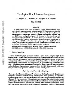
1.5 Multiple Views Bonsai provides a simple window manager that supports multiple scrollable images. Each window can display a different image, but windows can also be used to display different views of a complex structure. A view is considered to be a collection of graphical attributes and viewing parameters for the members of any set. Options are provided for binding the window to view a specific set, writing the current set out to a file or reading the contents of a file on to the set, and running filters on the set members. Sets can be viewed and filtered separately because graphical attributes are stored independently for each set. Consider a complex graph structure. Several views may be needed to reveal different aspects of the graph. One view might show the entire graph with the coordinates of its vertices positioned around the circumference of a circle to emphasize its rotational symmetry. A second view might show the same graph with its nodes repositioned to emphasize the structure of its component graphs. Each component could also be viewed in its own window with its own graphical attributes. These multiple views are possible because each Bonsai window can display a different set and each diagram element can appear in a different form in each set.

Figure 1. Multiple Views of a Complete Graph

-5-

1.6 Graphical Interface Bonsai’s graphical interface provides menus with options that invoke the same library of commands used by Bonsai’s parser. But rather than limiting the graphical interface to either prefix or postfix syntax, both are supported, because both are useful for different types of tasks. For a prefix syntax of graphical interaction: the type of command, or action, is first selected off a menu. Then the action can be applied to several items in succession. A postfix syntax of graphical interaction uses item-specific menus. An item is selected first, and then an action is chosen and applied to the item. Postfix syntax is useful for editing the diagram in local, specific ways, i.e., making one vertex small, another square, an edge label invisible, etc. Graphs and sets can be defined with a minimum of user input. Trees and paths of connected items can be defined with one menu selection and one mouse click for each new vertex; selecting a predefined vertex or set will start a new tree or path. Sets can be defined by either selecting a series of items in succession or sweeping a rectangle around a group of items. If both the source and destination items of an edge are members of the set, then the edge will become a member automatically. The set may not necessarily be shaped like a rectangle, even if it is defined by sweeping a rectangle. Diagram items are defined with default graphical attributes, which include shape, size, edge visibility, label visibility, color, etc. Separate defaults are stored for vertices, edges, and sets. Edges can connect predefined vertices and sets in either trees or paths. Edges can be displayed as splines by calculating an interpolation function through each of the spline’s control points. † Splines are useful for displaying graphs where more than one edge joins a pair of vertices, called multiple-adjacency, or where an edge connects a vertex to itself, a self loop; in either case, Bonsai automatically draws the splines so that they do not overlap. Additional control points can be added, and each control point can be repositioned to change the shape of the spline.

n0

n1

n4

n5

n7

n2

n3

n8

n6

n20

n21

n18

s0

n19

n9

n13

n10

n14

n11

n15

s3

s1 n16

Figure 2. Splines and Connected Trees, Paths, and Sets 1.7 Application Interface In order for Bonsai to be used as a graphical interface for an application, the application must not only send commands to a Bonsai input channel, but it must also watch for callback messages on a Bonsai output _______________ †

The code for computing quadric B-splines was supplied by Tom Duff.

-6-

channel. Callback messages in the current version of Bonsai are limited to errors, attribute information about graph items, and item and menu selections. A future version of Bonsai will either use X11 Widget callbacks 18 or allow applications to specify which Bonsai events are to be reported. Bonsai has a general method for handling errors and callbacks that attempts to deliver output to the appropriate process over the appropriate channel. For example, if an illegal command is generated on the standard input, an error will be reported on the standard output or if an illegal command is generated from an external process, the error will be sent back to that process on the appropriate socket. The graphical attributes and label of any item can be obtained by using the i command. Item selection is handled by storing the numeric id of the creating process’s channel with the item when it is created. Then when the item is selected, a callback message is generated on the appropriate channel. When an application menu is created with the Bonsai ‘‘menu’’ command, the id of the creating process’s channel is stored with the menu. Then when one of the options is selected from the application menu, a callback can be directed to the appropriate output channel. An application needs only a small amount of code to handle these callbacks and errors.

2. USING BONSAI FOR TOPOLOGICAL GRAPH THEORY Topological graph theory is not fundamentally different from other applications, but its requirements are of such a general nature that they revealed a few limitations of Bonsai’s design. These requirements will be introduced here and described further in the following sections. Whereas most other applications model data with graph diagrams, in topological graph theory, the objects of interest are the graphs themselves. Several basic graph structures have been identified by graph theorists. The basic graphs can be combined to form new graphs by applying a union operation. Several other graph operations can also be used to define new graphs from old ones. In topological graph theory, fundamental graph operations affect two or more graphs simultaneously and are often recursive. Many of the basic graphs are rotationally symmetric and can profit from graph layout techniques that maximize symmetry. Another requirement of topological graph theory is that all of the edges connected, or incident, to each vertex must have an unambiguous rotational order. Rotational ordering of incident edges is a variation of linear ordering, which is required by several other applications in order to compute graph layouts. † These requirements revealed limitations in Bonsai’s design. One limitation, which has been corrected, is that if more than one edge joined two vertices together, Bonsai would display the edges with the same endpoints. This meant that an unambiguous ordering of edges incident to a vertex could not be displayed or defined. Bonsai’s spline package has been redesigned to support rotational ordering. A circular layout algorithm that works with the new splines has been implemented to generate layouts that emphasize rotational symmetry. Other limitations that have not yet been corrected include: Bonsai’s language has no macro facility for interactive definition of new commands, Bonsai’s language has no provision for recursion, and Bonsai’s graphical interface does not allow interactive operations on more than one diagram element at a time. These limitations are being addressed in a new version of Bonsai. In the mean time, new commands have been added as primitives to Bonsai’s command language to support basic graph structures and operations. 2.1 Basic Graph Structures and Operations Commands have been added to Bonsai’s language to allow the generation of several basic graph structures: paths, cycles, bouquets, complete graphs, and cubes (see Figure 3). A path is a connected set of edges. In _______________ †

Linear ordering of incident edges may be determined by the application or by sorting application data associated with the incident edges or vertices. Typical orders include an alphanumeric sort of the labels of the incident vertices or a numeric sort of the creation timestamp of each incident vertex.

-7-

graph theory literature, basic graphs are indicated with a capital letter and a subscript that represents the number of vertices in the graph, or its order. For example, P n is a path of order n, which is n vertices chained together with n − 1 edges. In Bonsai, paths are specified with the P command, which requires an integer argument to indicate the path’s order. For example, P 4 will create a path with 4 vertices. A cycle is a path that starts and ends at the same vertex. The Bonsai command C 3 will create a cycle with 3 vertices and 3 edges. A bouquet is a vertex with several edge loops. The Bonsai command B 7 will create a vertex with 7 loops. Paths, cycles, and bouquets are all implemented with a C for-loop that either chains together edges and vertices (paths and cycles) or adds multiple edges to a single vertex (bouquets). In addition, these commands also generate a new set, which includes the vertices and edges of the new graph structure.

a b c

d

e

Figure 3. Basic Graphs: P4, C3, B7, K12, and Q4 In Bonsai, graphs are treated as sets: any graph can be bound to its own window and filtered separately from any other graph. Graphs can be passed as arguments to graph operations by passing the identifier of the set that represents the graph. Most graph operations take two graphs as arguments and create a third graph. The union of graph A and graph B, for example, is a new graph that has a set of vertices equal to the union of the vertices of A and B, and a set of edges equal to the union of the edges of A and B (see Figure 4). One problem associated with graph operations is indicating argument syntax in an interactive graphical interface. Most operations on Bonsai graphical objects are monadic and can be specified with the operand and operator in either order. Either an object is specified and then an action, or an action is specified and applied to several objects, one at a time. But graph operations have at least two input graphs to specify as well as the type of operation. Bonsai’s textual interface can easily handle commands with two operands, because object identifiers are the same as any other textual arguments. But handling syntax in a graphical interface is more complex than a textual interface. The interaction between code in different modules (the menu module and the direct-manipulation module) must be defined as well as certain end-user conventions such as the ‘‘current object’’ and the ‘‘current action’’. Supporting multi-operand commands with a graphical interface raises several questions, such as: Should infix order be supported? Can postfix order be

-8-

supported? How should operations with more than two operands be supported? These problem have not yet been addressed; the graph operations have only been implemented for Bonsai’s textual interface. Often a family of graphs is characterized by the recursive application of a primitive graph operation. Complete graphs, for example, can be created with the suspension operation. The suspension of two graphs is a new graph that is the union of both graphs and a new edge connecting each vertex in the first graph to each vertex in the second graph. The vertices of a complete graph are completely interconnected with edges. For example, the Bonsai command K 1 defines a complete graph of order 1, which is a single vertex; K 3 defines a triangle formed by three vertices and three edges. The K command is implemented through recursive calls to the suspension operation, sus. The suspension of any complete graph K n with K 1 is the next higher order complete graph. Cubes are also described operationally. The Cartesian product of a cube Q n with the complete graph K 2 is the next higher order cube, Q n + 1 . The cube command Q is implemented through recursive calls to the Cartesian product command, prod.

b a

c

d

e

Figure 4. Basic Graph Operations: Graph a, Graph b, union a b, sus a b, prod a b But Bonsai’s language has no provision for interactive definition of new primitive operations. When Bonsai was originally designed, it was thought that because external application programs can drive Bonsai’s interpreter with a text-stream, it would be easy for an application to define its own operations by invoking successive Bonsai commands and maintaining any state information that might be required between operations. If the union operation were implemented in a separate application program, for example, first two graphs would need to be passed to the application, which would compute the union, and the pass back the resulting new graph to be displayed in Bonsai. Bonsai’s parser and graph data structures are both written as libraries, which allows a certain amount of code to be shared, but does not circumvent the overhead involved in passing graphs between separate processes. Communication between processes can either be implemented by reading and writing files or through a pipe, socket, or stream. This approach would free Bonsai of any application-specific capabilities, but it has a high communication overhead. A more general solution would be to replace Bonsai’s command interpreter with a more powerful specification language, such as a variant of Scheme. 19 This would allow new commands to be added to

-9-

Bonsai by application programs. The new commands could access any previously defined commands and take full advantage of recursion. Programs like Emacs 20 and NeWs 21 gain a degree of extensibility by incorporating an interpreted extension language like Scheme or PostScript. Libraries of commands can be down-loaded to the interpreter to customize the capabilities of the running program. The implication of this approach is that it would require writing all extensions to Bonsai in whatever new extension language is chosen. Unfortunately this can have a negative effect on Bonsai’s usage if the extension language is perceived negatively by application developers. Even so, a future version of Bonsai will probably use some extension language in place of the current parser. For the current version of Bonsai, we chose a solution that is not general, but allowed us to quickly implement the desired functionality without sacrificing performance: we incorporated new C code directly into Bonsai to support basic graph structures and operations. We have made the assumption that structures and operations that are basic for graph theory will be useful for other applications as well. 2.2 Rotationally Symmetric Layout Several basic graph structures can benefit from a layout scheme that emphasizes rotational symmetry. A layout algorithm has been implemented that can be used to position either vertices or spline control points. Once the total number of vertices or control points to be positioned is calculated, they are spaced evenly around the circumference of a circle. Items are positioned in the order that they were defined in. Evenly spacing vertices along the circumference of a circle is suitable for cycles and complete graphs, while evenly spacing spline control points around a vertex is useful for drawing bouquets. The circle is centered at the average position of all the vertices or at the center of the single vertex in the case of a bouquet. This algorithm was used to create the layouts for Figure 3.b, 3.c, and 3.d. 2.3 Rotation Systems and Projections The objective of topological graph theory is to draw a graph on a surface so that no two edges cross. 22 Such a drawing is called an imbedding of a graph in a surface. Surfaces in topological graph theory are normally closed, which means finite and boundaryless like the surface of a sphere.† An imbedding on a closed surface can also be thought of as a segmentation of the surface into mutually exclusive regions or faces. Because no two edges of the graph can cross, each face is bounded by the edges of the graph. The vertices of the graph lie at the corners of each face. A closed surface can be stretched and deformed without changing the imbedding or, equivalently, without changing the number of faces and their relationship to each other. One technique for describing a graph imbedding is a combinatorial rotation system (hereafter called a rotation system). A rotation system is a graph with a cyclic ordering of edge-ends at each vertex. The cyclic ordering encodes the relationship between the corners of each face in the imbedding. There may be several different imbeddings of a graph in a given surface. Each imbedding corresponds to a different rotation system. Figure 5 shows a rotation system in textual form. Each line represents a vertex by its label and a ’.’ character followed by a list of incident edge (or vertex) labels. The order of labels is significant. It is the rotational order of edge connections at the vertex. The rotational direction (clockwise or counter-clockwise) is taken to be the same for all lists. Figure 5 indicates two vertices with three edge-ends each. In this case the vertices are multiply adjacent and vertex labels can not be used: edge labels are used to preserve the cyclic order. _______________ †

The surface of an infinite plane is boundaryless, but not finite; the surface of a disk is finite, but bounded by a circular edge; but the surface of a sphere has no bounding edge: it is compact and boundaryless, or closed.

- 10 -

n0. a0 a1 a2 n1. a0 a1 a2

Figure 5. Sample Rotation System

A 2-dimensional diagram of a rotation system is called a graphical rotation projection (hereafter called a rotation projection) because it is a 2-dimensional representation of a rotation system that might, in turn, be a representation of a higher order surface. It doesn’t matter if edges cross each other in a rotation projection: what matters is the unambiguous cyclic order of edge-ends at each vertex. Figure 6 shows a rotation projection for the rotation system of Figure 5.

a0 a1 n0

n1 a2

Figure 6. Graphical Rotation Projection for Figure 5. Figure 6 was defined as a graph diagram with Bonsai’s interactive graphical interface. The graph diagram is stored as a list of Bonsai commands as shown in Figure 7. Each line that begins with an ‘n’ defines a vertex and each line that begins with an ‘a’ defines an edge (Bonsai’s language is described in the Appendix). n n a a a

:i1 :i2 :s1 :s2 :s1

:x135 :y88 :x263 :y89 :d2 :l"a0" :d1 :l"a1" :d2 :l"a2"

:w14 :h14 :l"n0" :w14 :h14 :l"n1" :S198 :S110 :S351 :S55 :S31 :S30 :S134 :S24 :S263 :S160

Figure 7. Bonsai Diagram for Figure 5.

A rotation system captures more information that a generic graph and less than a layout. A generic graph can be represented as a set of vertices with sets of incident edges; no ordering information is associated with the vertices or edges. A graph layout has additional information consisting of spatial coordinates for each vertex; edge coordinates can be computed from the graph connectivity and the vertex coordinates. But a rotation system imposes a cyclic order on the incident edges: it implies a set of possible layouts without specifying specific coordinates. Bonsai diagrams could be used as rotation projections if the cyclic order of edges at each vertex could be unambiguously determined. Unfortunately, one of the assumptions made while implementing Bonsai’s splines limited the connection point between edges and vertices. This design assumption allowed the same endpoints stored for straight edges to be used for splines, but it meant that a spline could not be used to curve around a vertex and connect to its far side — an important requirement for drawing and editing rotation projections.

- 11 -

To solve this problem, Bonsai’s splines were modified. A new subroutine was created that takes a point and a vertex as arguments, and returns the point on the vertex’s border that is closest to the input point. This subroutine is used to recalculate arc endpoints for straight line edges and splines. Now a spline begins at the point on the source vertex’s border that is closest to the first control point. A spline ends at the point on the destination vertex’s border that is closest to the last control point. Even the new splines can’t solve all the problems of graphical ambiguity: edges and vertices can be positioned to lie directly on top of each other. It remains up to the user to position splines carefully when editing rotation projections with the graphical interface. Another potential problem is that rotation systems may not be preserved by vertex repositioning. It would be a mistake for a user to assume that editing a rotation projection to make it look a bit simpler and nicer might not change it into a projection of a different rotation system. Perhaps it is better to view this as an advantage: several related rotation systems can be quickly generated from the same graph by merely repositioning vertices or spline control points. In addition to redesigning the splines, Bonsai’s language was also extended to encode spline control points (this had been previously unimplemented). Now splines can be defined and edited textually, saved in text files, and passed to separate filter programs. In particular, a small filter program, called bon2rot, has been written to convert Bonsai graph files into rotation systems. A second filter, rot2bon, converts rotation systems back into Bonsai’s language. 2.4 Converting Bonsai Diagrams into Rotation Systems Figure 8 shows the pseudo code for the bon2rot algorithm, which converts coordinate information into a sorted list of incident edges.† It uses a data structure, Rot, which holds an angle and an edge pointer. The algorithm for parsing the Bonsai input file is a straightforward implementation of a tokenizer and dispatch table that is not described here. The expensive part of the bon2rot algorithm is the angle sort at each vertex with more than 2 incident edges.

_______________ †

In this paper algorithms are described as a collection of descriptive comments with a C-like syntax.

- 12 -

parse bonsai file; for(each vertex){ print its label and a ’.’; count incident edges including loops; if(there are 1 or 2 edges){ for(each edge){ if(arc labels) print arc label; else find dest vertex and print its label; } } else{ make array of rots one per edge; for(each edge){ if(spline) calculate angle from atan of line segment from center of vertex to next control point; else calculate angle from atan of line segment from center of vertex to center of incident vertex; } sort rots by angle; if(arc labels) print arc label; else print vertex labels; } }

Figure 8. Pseudo Code for the bon2rot Algorithm

2.5 Converting Rotation Systems into Bonsai Diagrams Converting rotation systems into rotation projections is a one-to-many mapping: several diagrams can be generated by a single rotation system description. Because a rotation system includes no information about node or arc coordinates, the layout of the rotation projection must be calculated. Although creating a layout that preserves a rotation system is straightforward, creating a layout that looks ‘‘nice’’ and ‘‘simple’’ is very difficult. Graph layout is such a difficult and application-dependent problem that our approach would normally be to create a separate filter program for computing layouts of rotation projections. In this case, however, we have taken a shortcut and included a naive solution to the rotation system layout problem directly in the rot2bon filter.

- 13 -

parse rotation system; for(each vertex in rotation system){ position vertex; determine valence of incident edges; assign positions of spline control points of incident edges such that the control points lie on the circumference of a circle around the vertex (position the first control point of out-edges, the second of in-edges); } print out Bonsai file;

Figure 9. Pseudo Code for rot2bon Algorithm

The pseudo code for the rot2bon algorithm is shown in Figure 9. This program implements a naive layout by positioning vertices at arbitrary grid-points paying no attention to their connectivity. Each spline is defined with two interior control points. Each vertex is positioned with the closest control points of its incident splines. The other end of the splines are positioned with a different vertex. It generates ‘‘correct’’ projections in that a vertice’s incident arcs radiate outward in the proper relative order, but it relies on the spline’s interpolation function to draw the midpoints of the splines, which has unpredictable results. Designing a parser for rotation systems is a clearer problem to solve, but it has a few surprising subtleties. One is related to the fact that edges are indicated twice: once for each adjacent vertex. The general strategy is to build a graph structure while parsing the rotation system, but because edges are indicated twice, they are only added to the graph after both of their incident vertices have been parsed. The exception to this rule is edges that are loops, because a loop has only one incident vertex. Another complication is that the labels used to indicate incidence may be edge labels or vertex labels. The pseudo code for the parser is shown in Figure 10.

- 14 -

for(each line of input){ get the label of the initial vertex; if(its already in the graph) root = vertex; else{ add a new vertex to the graph; root = new vertex; } for(all other tokens on input line){ if(edge labels){ if(edge label is not in list) add edge to list; else /* this is the second end of edge */ add edge to graph; } else{ /* vertex labels */ if(vertex is already in the graph){ if(vertex == root) /* a loop */ add edge to graph; else if((token + root’s label) is not in list){ add edge to graph; add (root’s label + token) to list; } } else{ /* vertex is not in the graph */ add a new vertex to the graph; add a new edge to the graph; add (root’s label + token) to list; } } } }

Figure 10. Pseudo Code for Rotation System Parser

If edge labels are used to indicate incidence, a list is kept of edge labels as they are parsed. An edge is only added to the graph if it already appears in the list, which means that the second end of the edge is being parsed. Keeping a list of edge labels is inefficient, but it is used anyway because it is particularly convenient for storing vertex labels. If vertex labels are used to indicate incidence, the algorithm is more complicated. A list of strings is still kept, but the strings are not just the vertex labels, but a concatenation of the first vertex label on the input line with each other token on the line. The concatenated labels are needed to find the correct edge. Storing the vertex labels alone is insufficient because it takes two vertices to identify an edge (except for loop edges). To determine if the first end of an edge has been parsed the list is checked for the string (token + root’s label). If that string is not in the list, the string (root’s label + token) is added to the list. This is because when parsing the input line that corresponds to the other end of the edge, the root’s label and the token will be reversed.

- 15 -

2.6 Orientation and Imbedding Distributions Additional programs have been created to support some of the more complex operations required by topological graph theory. These programs can be used to compute characteristics of graphs and the surfaces that they can be imbedded in. One important characteristic of a surface is its orientation. Closed surfaces can be either orientable or non-orientable. The surface of the earth, for example, is orientable because it can have a coordinate system such that each coordinate maps to only one point on the surface. Non-orientable surfaces do not have the property that a coordinate system can define all points uniquely. .. One non-orientable surface is the Mobius band, which can be modeled with a long flat strip joined at the ends with a half-twist. The twist reverses the orientation of the surface, which prevents any coordinate system from being able to describe surface points unambiguously. The twist also causes the band to have only one edge, which is a deformed circle. Like surfaces, graphs can be orientable or non-orientable. A non-orientable graph can not be imbedded on an orientable surface. Graphs can have orientation-reversing edges (hereafter called twisted edges). Even graphs with several twisted edges may be orientable because two twists cancel each other: only edges with an odd number of twists are considered twisted. The algorithm in Figure 11 can be used to reduce a graph to its minimum number of twisted edges. Twisting each of the destination vertex’s edges has the sideeffect of untwisting the edge that was just crossed. The spanning tree, therefore, will contain no twisted edges after it has been traversed. Twisting each of a vertex’s edges is an operation that preserves the graph’s orientation; it is equivalent to reversing the rotational order of the vertex. 22

while(walking any spanning tree of the graph) if(any twisted edge is crossed) twist each of the destination vertex’s edges; if(any twisted edges remain in the graph) the graph is non-orientable; else the graph is orientable;

Figure 11. Pseudo Code for rot2or Orientation Reduction

The rot2or program is an implementation of the orientation reduction algorithm, which can be used to determine the orientation of a rotation system. Twisted edges are indicated with a single quote as the last character of their label. This convention allows any edge defined with Bonsai to be marked as twisted by editing its label. One detail excluded from the description of the rotation system parser in Figure 10, is that it checks to see if each edge is twisted and stores the orientation internally. This allows rot2or to use the same parser without losing the orientation information of each edge. Another way to characterize a surface is by its genus. A surface’s genus can be thought of as its number of tunnel-like holes. For example, the surface of a doughnut, also called a torus, has genus of 1: it is thought of as a spherical surface with one tunnel-like hole through it. A sphere has a surface with a genus of 0. A double-torus (a sphere with 2 holes) has a surface of genus 2. A graph that can be imbedded on a spherical surface can also be imbedded on a surface of higher genus such as the surface of a torus. For any graph, there is a surface of minimum genus required for the imbeddeding (hereafter called the imbedding surface). A procedure called face-tracing can be used to count the faces that are implied by a rotation system and this

- 16 -

number can be used to determine the imbedding surface. Faces are related to genus by a generalization of Euler’s equation relating the numbers of vertices, edges and faces of a spherical polyhedron (see Equation 1). The right-hand side of Equation 1, called the Euler characteristic, can be generalized to non-spherical surfaces as shown in Equation 2, where g equals the genus of the imbedding surface. 22 Equation 2 indicates that given a rotation system with a fixed number of vertices and edges, only the number of faces is required to compute the genus of the imbedding surface. V −E +F =2

(1)

V − E + F = 2 − 2g

(2)

A program called rot2face performs the face-tracing algorithm on a rotation system and determines the implied imbedding surface. Three new data structures were defined to implement rot2face: a corner is two edges and a vertex, a face is a list of corners, and a surface is a list of faces. All the complexity in the rot2face program is in the face-tracing algorithm, shown in Figure 12. Once the rotation system is parsed, a Corner structure is filled for each pair of adjacent edges. Then a corner is selected that is not yet in the Surface, and a face is traced for that corner. The pathtype variable stores the cumulative orientation of edges in the face and is used to select the next edge in the face. When tracing along an edge and arriving at a new vertex, the next edge in the face is the edge incident to the new vertex that is next in the clockwise edge order if the pathtype is not twisted. If the pathtype is twisted, however, the next edge in the face is the one previous in the clockwise edge order (or next in counter-clockwise order).

cp = the first corner in the face; for(;;){ edge2 = cp->edge2; pathtype += edge2’s orientation; find edge2’s destination vertex; if(edge2 is a loop) edge1 = other end of loop; else edge1 = edge incident to destination vertex with the same label as edge2; if(pathtype % 2) /* path is twisted */ edge2 = edge counter-clockwise-adjacent to edge1; else /* path is not twisted */ edge2 = edge clockwise-adjacent to edge1; cp = a new corner with edge1, destination vertex, and edge2; if(cp == the first corner in the face) return; }

Figure 12. Pseudo Code for Face Tracing

For several graphs, each of the possible different rotation systems and their corresponding imbedding surfaces can be computed. The list of surfaces is called the genus distribution of the graph and it can be calculated with a program called bon2gdist. Genus distributions for a few basic graphs are shown in Table 1. For large graphs, or graphs with many edges, it may be computationally impractical to compute the genus distribution. For these graphs it is useful to generate several random rotation systems and compute their

- 17 -

imbedding surfaces. A list of surfaces generated in this way is called a random genus distribution and it can be calculated with a program called bon2grand.

Table 1. Genus Distributions of a few Basic Graphs ____________________________________________ ____________________________________________ Graph  genus 0  genus 1  genus 2  total  ____________________________________________   B2  4  2  6  ____________________________________________      B3  40  80  120  ____________________________________________  ____________________________________________ B4  672  3360  1008  5040        B 5  16128  161280  185472  362880  ____________________________________________ ____________________________________________  K4  2  14  16   K     462  4974  2340  7776  5  ____________________________________________ Calculating all the possible rotation systems of a graph is equivalent to finding all the combinations of all the permutations of edges incident to each vertex. If a vertex has a valence of k, then there are ( k − 1 ) ! possible permutations of incident edges. Each vertex permutation must be combined with all others. A graph with V k-valent vertices, for example, has ( (k − 1 ) ! ) V possible rotation systems. We use a variation of Johnson’s permutation algorithm 23 that returns permutations on demand without performing factorial division or recursion. Obtaining permutations on demand is desirable when computing genus distributions because it saves space during the computation, which allows the calculation to be performed for larger graphs. Like Johnson’s algorithm, successive permutations are computed by interchanging two adjacent elements of the previous arrangement. The pseudo code for the bon2gdist algorithm is shown in Figure 13. After catching a UNIX SIGQUIT signal, the bon2gdist program invokes its cleanup() routine which prints the frequency counts of each genus before quitting. When handling a SIGINT signal, the cleanup() routine prints the frequency counts and continues processing so that users can check on partial results without stopping the calculation. In order to perform the face tracing calculation, the graph structure must be arranged according to the current set of permutations. This has been optimized somewhat with a subroutine that rebuilds a vertex’s list of edges in an order specified by the permuted list of edge labels.

- 18 -

parse Bonsai file; build graph for face tracing; build edge label and flag arrays; sort edge label arrays; for(j = 0; ; ){ if(there is not another permutation for vertex j) cleanup(); j++; for(k = 0; k < j; k++){ reset lists for all vertices < j; reset graph structure for all vertices < j; } reset graph structure for vertex j; build and count faces; calculate genus and store result; free surface; cleanup(); }

Figure 13. Pseudo Code for bon2gdist Algorithm

Calculating the genus distribution of graphs can be impractical. Knuth suggests that any algorithm with more than 10 ! calculations may be impractical to implement on a computer. 24 One example of a small graph with an impractical genus distribution calculation is B 6 , a bouquet with one vertex and 6 self-loops. B 6 has 11 ! possible permutations because its vertex has 12 edge-ends. It is possible to approximate a genus distribution calculation by selecting successive random rotation systems and computing their genus. We make the assumption that because the genus distribution is large, it is unlikely that repeated selection of the same rotation system will affect our calculations. The bon2grand program takes three optional arguments: one is the total number of random rotation systems to generate, which defaults to 500, the second is a seed for the random number generator, which allows the same calculation to be repeated, and the third is a flag for verbose operation. The pseudo code for bon2grand is shown in Figure 14. The nrand(n) command returns a random number in the range of 0 ≤x < n. Like bon2gdist, signals are handled to print partial results without stopping the calculation.

- 19 -

parse Bonsai file; build graph for face tracing; check validity of optional total argument; build edge label and flag arrays; sort edge label arrays; seed random number generator; for(j = 0; j < total; j++){ for(each vertex){ if(!nrand(2)) /* flip a coin */ continue; if(!v = vertex valence) /* no incident edges continue; swap edge label nrand(v) with adjacent edge label; reset graph structure for vertex; } build and count faces; calculate genus and store result; free surface; } cleanup();

*/

Figure 14. Pseudo Code for bon2grand Algorithm

One other program has been implemented, bon2xdist, which calculates the crosscap distribution of a graph. .. A crosscap can be thought of as a circular hole removed from a surface and replaced with a Mobius band. This substitution is hard to imagine because it is impossible in 3-dimensional space. A sphere with one crosscap is equivalent to any closed surface with a crosscap number of 1. The crosscap number can be thought of the total number of orientation-reversing regions on a surface: a graph with n twisted edges can be imbedded on a surface with n crosscaps. To calculate a graph’s crosscap distribution, each of the different rotation systems must be considered for each combination of twisted and non-twisted edges. We apply the result of the orientation reduction algorithm (see Figure 11) to eliminate consideration of all edges in a random spanning tree of the graph. If there are n edges in the graph that are not in the spanning tree, then there are 2 n possible combinations of twisted and untwisted edges to consider. The pseudo-code for bon2xdist is shown in Figure 15. Crosscap distributions for two basic graphs are shown in Table 2.

- 20 -

parse Bonsai file; build graph for face tracing; twistset = set of all edges not in a spanning tree of graph; build edge label and flag arrays; sort edge label arrays; for(each combination of twists in twistset){ for(j = 0; ; ){ if(there is not another permutation for vertex j) break; j++; for(k = 0; k < j; k++){ reset lists for all vertices < j; reset graph structure for all vertices < j; } reset graph structure for vertex j; build and count faces; calculate crosscap and store result; free surface; } reset all lists; } cleanup();

Figure 15. Pseudo Code for bon2xdist Algorithm

Table 2. Crosscap Distributions of Two Bouquets _____________________________________________ ______________________________________________ Graph  twisted edges  crosscap 0  crosscap 1  ____________________________________________     B2  0 4 2      1 8 4      2 4 2 _____________________________________________         B3  0 40 80      1 120 240      2 120 240      3 40 80 _____________________________________________    

3. FUTURE WORK One extension of this work would be to compute and display graph imbeddings on 3-dimensional surfaces. This would be particularly challenging for non-orientable surfaces. One strategy would involve computing a layout on a rectangular surface and using coupled cylindrical projections to map the rectangle to the surface of a torus. The layout algorithm would need to handle the identity of opposite edges of the rectangle. This could be generalized for all orientable surfaces by computing layouts on several rectangles with rectangular holes, but this would require a more complex layout algorithm. 25

- 21 -

Several of the lessons learned from topological graph theory have helped to shape plans for redesigning Bonsai. A new version of Bonsai has been prototyped, which runs only on X Windows. The C++ graph library is used to store Bonsai’s graph data structures and handle set operations, but the library has no notion of ordered sets. A new graph library is being designed to support application-specific ordering of set members. This will provide a general solution for supporting rotational orderings of edges and linear orderings for layout. Several other problems need to be addressed including selection of an extension language, improving the application interface, and handling of multiple operands in the graphical interface. Bonsai is being extended in several other directions. Graph layout is known to be a hard problem, but one that often has simplifications for particular applications. There is currently an interest in layout algorithms for software data structure diagrams, which can probably benefit from a hierarchical strategy. There is also the problem of efficient layout algorithms for interactively changing graphs. Additional viewing and navigation filters need to be implemented to address the problems involved in understanding complex timevarying structures.

4. CONCLUSION A generalized graph browser system has been extended for topological graph theory. The requirements of topological graph theory have revealed some problems with the design of the browser, which will bare on its reimplementation. Several additional programs have been described for computing various characteristics of graphs and their imbedding surfaces. Together with the browser these programs provide an environment for exploring topological graph theory that leverages the diagrammatic representation of graphs with the interactive graphics capabilities of computer workstations.

5. ACKNOWLEDGMENTS This work would not have been possible without the support of Bell Laboratories and Columbia University. Several people have provided advice and input including: Beth Craig, Tom Duff, Mark Jones, Ted Kowalski, Doug McIlroy, Larry Ruedisueli, Jonathan Shopiro, and Mike Wish. Att. References Appendix

- 22 -

REFERENCES [1] Potmesil, M. and Hoffert, E. M., ‘‘FRAMES: Software Tools for Modeling, Rendering and Animation of 3D Scenes,’’ Computer Graphics 21(4), pp. 85-95 (July 1987). [2] Haeberli, P. E., ‘‘ConMan: A Visual Programming Language for Interactive Graphics,’’ Computer Graphics 22(4), pp. 103-111 (August 1988). [3] Stellar Computer, Application Visualization System Users’ Guide, Release 2, Newton, MA (November 20, 1989). [4] Rowe, L. A., Davis, M., Messinger, E., Meyer, C., Spirakis, C., and Tuan, A., ‘‘A Browser for Directed Graphs,’’ Software-Practice and Experience 17(1), pp. 61-76 (January 1987). [5] Newberry, F. J., ‘‘An Interface Description Language for Graph Editors,’’ 1988 IEEE Workshop on Visual Languages, pp. 144-149, IEEE Computer Society Press (October 10-12, 1988). [6] Robins, G., The ISI Grapher, Information Sciences Institute, Intelligent Systems Division, Marina Del Rey, California (June 10, 1987). [7] Helfman, J. I., Bonsai Users’ Guide, AT&T Bell Laboratories internal memorandum (September 15, 1989). [8] Kernighan, B. W. and Ritchie, D. M., The C Programming Language, Prentice-Hall, Inc., Englewood Cliffs, New Jersey (1978). [9] Pike, R., ‘‘The Blit: A Multiplexed Graphics Terminal,’’ AT&T Bell Laboratories Technical Journal 63(8 Pt. 2), pp. 1607-1631 (October 1984). [10] Sun Microsystems, Incorporated, SunView 1 System Programmer’s Guide, Mountain View, California (May 9, 1988). [11] Scheifler, R. W. and Gettys, J., ‘‘The X Window System,’’ ACM Transactions on Graphics 5(2), pp. 79-109 (April, 1986). [12] Kapilow, D. A. and Helfman, J. I., A 5620 Emulator Library for Version 11 X Windows and Suntools, AT&T Bell Laboratories internal memorandum (May 25, 1988). [13] Stroustrup, B., The C++ Programming Language, Addison-Wesley (1986). [14] Harel, D., ‘‘On Visual Formalisms,’’ Communications of the ACM 31(5), pp. 514-530 (May 1988). [15] Adobe Systems Incorporated, PostScript Language Reference Manual, Addison-Wesley, Reading, Massachusetts (1987). [16] Kernighan, B. W., ‘‘PIC - A Graphics Language for Typesetting,’’ CSTR 116, Bell Laboratories (1984). [17] Furnas, G. W., ‘‘Generalized Fisheye Views,’’ Human Factors In Computing Systems, CHI’86 Proceedings, pp. 16-23, Mantei, M. and Orbeton, P. (Eds.), ACM/SIGCHI (April 13-17, 1986). [18] Swick, R. R. and Weissman, T., X Toolkit Widgets - C Language X Interface, X Window System, X Version 11, Release 2, Digital Equipment Corporation, Massachusetts Institute of Technology (1988). [19] ‘‘Revised3 Report on the Algorithmic Language Scheme,’’ SIGPLAN Notices 21(12), pp. 37-79 (December 1986). [20] Stallman, R. M., ‘‘EMACS: The Extensible, Customizable, Self-Documenting Display Editor,’’ ACM SIGPLAN SIGOA Symposium of Text Manipulation, pp. 147-156, ACM, Portland, Oregon (June 1981).

- 23 -

[21] Gosling, J., Rosenthal, D., and Arden, M., The NeWs Book: An Introduction to the Network/extensible Window System, Springer-Verlag (1989). [22] Gross, J. L. and Tucker, T. W., Topological Graph Theory, Wiley-Interscience, John Wiley & Sons, New York (1987). [23] Johnson, S. M., ‘‘Generation of Permutations by Adjacent Transposition,’’ Mathematics of Computation 17(83), pp. 282-285 (July 1963). [24] Knuth, D. E., The Art of Computer Programming: Volume 1/Fundamental Algorithms, AddisonWesley, Reading, Massachusetts (1973). Second edition, p. 46. [25] Duff, T., personal communication.

- 24 -

Appendix: Bonsai’s Command Language

In Figure 17, all the Bonsai commands are shown in verbose form, with non-optional arguments in default order and with (redundant) prefixes. Optional arguments are shown enclosed in square braces. The ’˜’ character indicates one of the graphical attribute keywords listed in Figure 16. Some attribute keywords are aliases of each other (shown separated by a ’’). Most attribute keywords only affect items of a certain type (shown by a note in square braces). The ’*’ character indicates an item specification (either a number or a label). The ’#’ character indicates an integer. The ’%’ character indicates a string. Strings should be enclosed in double quotes if they include spaces or begin with a digit. The ‘‘...’’ string indicates that multiple arguments are possible of the preceding type. For example, ‘‘:o˜ ...’’ indicates that multiple graphical attribute options are possible.

box circle ellipse large  big small solid  e_on invis  e_off l_on l_off a_on a_off s_on s_off

make item a box [nodes and sets] make item a circle [nodes and sets] make item an ellipse [nodes and sets] make item big [nodes and sets] make item small [nodes and sets] make item’s border visible [nodes and sets] make item’s border invisible [nodes and sets] make item’s label visible make item’s label invisible make arrow visible [arcs] make arrow invisible [arcs] make spline visible [arcs] make spline invisible [arcs]

Figure 16. Graphical Attribute Keywords

B :n# [:i# :x# C :n# [:i# :x# K :n# [:i# :x# P :n# [:i# :x# Q :n# [:i# :x# a :s* :d* [:l% bind :i# :s* bw :i# circle :i* :s* clear d [:a˜ ... :n˜ dag [:h]

:y# :y# :y# :y# :y# :i#

:w# :w# :w# :w# :w# :o˜

:h# :h# :h# :h# :h# ...

[:f]

:l% :l% :l% :l% :l% :f]

... :s˜ ...]

:o˜ :o˜ :o˜ :o˜ :o˜

... ... ... ... ...

:f] :f] :f] :f] :f]

define a bouquet of n circles define a cycle of length n define a multiply connected graph define a path of length n define a cube of dimension n add an arc bind a window to a subset move a window to the bottom invoke circular layout algorithm remove all graph items from current set assign item defaults invoke dag layout algorithm

- 25 -

e :s* :i* ez :s* :i* f [* ...] fe * [* ...] i :i* [:x :y :w :h :l :o] menu % [% ...] n :i# [:x# :y# :w# :h# :l% :o˜ ... :f] namespace [:i*] o % p % prod :s* :d* [:i# :x# :y# :w# :h# :l% :o˜ ... :f] q r :i* [:x# :y# :w# :h# :l% :o˜ ... :f] rd * [* ... :f] rw :i# [:x# :y# :w# :h#] s :i* [:x# :y# :w# :h# :l% :o˜ ... :f] sleep # sus :s* :d* [:i# :x# :y# :w# :h# :l% :o˜ ... :f] tile tw :i# union :s* :d* [:i# :x# :y# :w# :h# :l% :o˜ ... :f] w :i# [:x# :y# :w# :h#] x * [* ... :f] xs :s* [:f] xw :i#

Figure 17. Bonsai Commands

add an item to a set remove an item from a set fix/redraw items, if no args redraws entire graph erase items get info about items add an application menu add a node, same as r if index already exists bind channel commands to new namespace open a file and read it onto current set put the current set out to a file define the vector product of two sets quit Bonsai reshape an item reshape items to the current defaults reshape a window add a set suspend process define the suspension of two sets invoke tile layout algorithm move a window to the top define the union of two sets add a window delete items delete a set and all its members delete a window