Extending LargeRDFBench for Multi-Source Data at Scale for SPARQL Endpoint Federation Ali Hasnain1 , Muhammad Saleem2 , Axel-Cyrille Ngonga Ngomo23 , and Dietrich Rebholz-Schuhmann1 1
Insight Centre for Data Analytics, National University of Ireland, Galway
[email protected] 2 Universit¨ at Leipzig, IFI/AKSW, PO 100920, D-04009 Leipzig
[email protected] 3 DICE, University of Paderborn, Germany
[email protected] Abstract. Querying the Web of Data is highly motivated by the use of federation approaches mainly SPARQL query federation when the data is available through endpoints. Different benchmarks have been proposed to exploit the full potential of SPARQL query federation approaches in real world scenarios with their limitations in size and complexity. Previously, we introduced LargeRDFBench - a billion-triple benchmark for SPARQL query federation. In this work, we pinpoint some of of the limitation of LargeRDFBench and propose an extension with 8 additional queries. Our evaluation results of the state-of-the-art federation engines revealed interesting insights, when tested on these additional queries.
1
Introduction
Due to linked, autonomous, and decentralised architecture of Linked Open Data (LOD), several queries require collecting information from more than one dataset also called data sources [8]. Processing such queries called federated queries are of central importance for the scale-able deployment of Semantic Web technologies. The importance of federated SPARQL queries for Linked Data management has led to the development of several federated SPARQL querying federation engines [12,1,14,5,7,10] etc. Consequently, this has motivated the design of several federated SPARQL querying benchmarks [9,13,6]. LargeRDFBench [9] addressed several limitation of FedBench [13] and Splodge [6]. In this work, we highlight some of the limitations of LargeRDFBench. In particular, the number of distinct datasets (sources for short) required to get the complete result set of the query is smaller in number (range between 1-4). As such, federation engines (e.g., [15]) which optimise the ordering of the required distinct sources explicitly mentioned as SPARQL SERVICES cannot be fully tested with existing LargeRDFBench queries. To fill this gap, we extended the LargeRDFBench with 8 additional queries of varying complexities and number of distinct sources required. We discussed the key characteristics of each of these additional queries and evaluated state-of-the-art engines on these queries. The evaluation results revealed interesting insights about the performance and stability of these engines. The LargeRDFBench along with the proposed extension is available at: https://github.com/AKSW/largerdfbench.
2
Related Work
Over the last decade, various benchmarks have been proposed for comparing triple stores and SPARQL query processing systems. In this work, we only focus on federated SPARQL queries benchmarks. SPLODGE [6] benchmark uses heuristic for automatic generation of federated queries with conjunctive BGPs. Non-conjunctive queries that make use of the SPARQL UNION, OPTIONAL clauses are not considered. FedBench [13] comprise of 9 real-world datasets and a total of 25 queries from different domains. Some of the limitations of FedBench was addressed in LargeRDFBench [9] with more real-world datasets and more complex and large data queries. In this work, we addressed some of the key limitations of LargeRDFBench and proposed an extension to this benchmark.
3
Design Features
In this section, we present the key SPARQL query features that should be considered while designing a federated SPARQL benchmark. Note that all of these key SPARQL features are formally presented in LargeRDFBench [9]. Here, we are re-introducing all of them for the sake of self containment of this paper and understanding the subsequent analysis. The previous research contributions [6,9] on SPARQL querying benchmarking pointed out that SPARQL queries used in the benchmark should vary with respect to the the following key query characteristics: total number of triple patterns, number of join vertices, mean join vertex degree, number of sources span, query result set sizes, mean triple pattern selectivities, BGP-restricted triple pattern selectivity, join-restricted triple pattern selectivity, join vertex types (‘star’, ‘path’, ‘hybrid’, ‘sink’), and important SPARQL clauses used (e.g., LIMIT, OPTIONAL, UNION, FILTER etc.). We represent any basic graph pattern (BGP) of a given SPARQL query as a directed hypergraph (DH) [11], a generalisation of a directed graph in which a hyperedge can join any number of vertices. In our specific case, every hyperedge captures a triple pattern. The subject of the triple becomes the source vertex of a hyperedge and the predicate and object of the triple pattern become the target vertices. For instance, the query (Figure 1) shows the hypergraph representation of a SPARQL query. Unlike a common SPARQL representation where the subject and object of the triple pattern are connected by an edge, our hypergraph-based representation contains nodes for all three components of the triple patterns. As a result, we can capture joins that involve predicates of triple patterns. Formally, our hypergraph representation is defined as follows: Definition 1 (Directed hypergraph of a BGP). The hypergraph representation of a BGP B is a directed hypergraph HG = (V, S E) whose vertices are all the components of all triple patterns in B, i.e., V = (s,p,o)∈B {s, p, o}, and that contains a hyperedge (S, T ) ∈ E for every triple pattern (s, p, o) ∈ B such that S = {s} and T = (p, o). The representation of a complete SPARQL query as a DH is the union of the representations of the query’s BGPs. Based on the DH representation of SPARQL queries, we can define the following features of SPARQL queries:
SELECT DISTINCT * WHERE { ?drug :description ?drugDesc. ?drug :drugType :smallMolecule. ?drug :keggCompoundId ?compound. ?enzyme :xSubstrate ?compound. ?chemReaction :xEnzyme ?enzyme. ?chemReaction :equation ?chemEquation. ?chemReaction :title ?reactionTitle }
Fig. 1: DH representation of the SPARQL query
Definition 2 (Join Vertex). For every vertex v ∈ V in such a hypergraph we write Ein(v) and Eout(v) to denote the set of incoming and outgoing edges, respectively; i.e., Ein(v) = {(S, T ) ∈ E | v ∈ T } and Eout(v) = {(S, T ) ∈ E | v ∈ S}. If |Ein(v)| + |Eout(v)| > 1, we call v a join vertex. Definition 3 (Join Vertex Types). A vertex v ∈ V can be of type “star”, “path”, “hybrid”, or “sink” if this vertex participates in at least one join. A “star” vertex has more than one outgoing edge and no incoming edges. A “path” vertex has exactly one incoming and outgoing edge. A “hybrid” vertex has either more than one incoming and at least one outgoing edge or more than one outgoing and at least one incoming edge. A “sink” vertex has more than one incoming edge and no outgoing edge. A vertex that does not participate in joins is “simple”. Definition 4 (Number of Join Vertices). Let ST ={st1 ,. . . , stj } be the set of vertices of type ‘star’, P T ={pt1 ,. . . , ptk } be the set of vertices of type ‘path’, HB ={hb1 ,. . . , hbl } be the set of vertices of type ‘hybrid’, and SN ={sn1 ,. . . , snm } be the set of vertices of type ‘sink’ in a DH representation of a query, then the number of join vertices in the query #JV = |ST | + |P T | + |HB| + |SN |. The total number of join vertices in a query is the sum of the total number of join vertices across all of the BGPs contained in this query. Definition 5 (Join Vertex Degree). The DH representation of SPARQL queries makes use of the notion of Ein (v) ⊆ E and Eout (v) ⊆ E to denote the set of incoming and outgoing hyperedges of a vertex v. The join vertex degree of a vertex v is denoted JV Dv = |Ein (v)| + |Eout (v)|. The join vertex degree of the complete query is the average of all join vertex degrees of all the joins contained in this query. In our example (see Figure 1), the number of triple patterns is seven and the number of join vertices is four (two star, one sink and path each). The join vertex degree of each of the ‘star’ join vertex (shown in green colour) given in Figure 1 is three (i.e., three outgoing hyperedges from both vertices). Definition 6 (Relevant Source Set). Let D be the set of all data sources (e.g., SPARQL endpoints), T P be the set of all triple patterns in query Q. Then,
a source d ∈ D, is relevant (also called capable) for a triple pattern tpi ∈ T P if at least one triple contained in d matches tpi .4 The relevant source set Ri ⊆ D for tpi is the set that contains all sources that are relevant for that particular triple pattern. Definition 7 (Total Triple Pattern-wise Sources). By using Definition 6, we can define the total number of triple pattern-wise sources selected for query Q as the sum of the magnitudes of relevant source sets Ri over all individual triple patterns tpi ∈ Q. Definition 8 (BGP-Restricted Triple Pattern Selectivity). Consider a Basic Graph Pattern BGP and a triple pattern tp i belonging to BGP , let R(tpi , D) be the set of distinct solution mappings (i.e., resultset) of executing tpi over dataset D and R(BGP , D) be the set of distinct solution mappings of executing BGP over dataset D. Then the BGP-restricted triple pattern selectivity denoted by Sel BGP−Restricted (tpi , D) is the fraction of distinct solution mappings in R(tpi , D) that are compatible (as per standard SPARQL semantics [3]) with a solution mapping in R(BGP , D) [2]. Formally, if Ω and Ω 0 denote the sets underlying the (bag) query results R(tp i , D) and R(BGP , D), respectively, then Sel BGP−Restricted (tpi , D) =
|{µ ∈ Ω |∃µ0 ∈ Ω 0 : µ and µ0 are compatible}| |Ω|
Definition 9 (Join-Restricted Triple Pattern Selectivity). Consider a join vertex x in the DH representation of a BGP . Let BGP 0 belonging to BGP be the set of triple patterns that are incidents to x. Furthermore, let tpi belonging to BGP 0 be a triple pattern and R(tpi , D) be the set of distinct solution mappings of executing tpi over dataset D and R(BGP 0 , D) be the set of distinct solution mappings of executing BGP 0 over dataset D. Then the x − restricted triple pattern selectivity denoted by SelJVx−Restricted (tpi , D), is the fraction of distinct solution mappings in R(tpi , D) that are compatible with a solution mapping in R(BGP 0 , D) [2]. Formally, if Ω and Ω 0 denote the sets underlying the (bag) query results R(tp i , D) and R(BGP 0 , D), respectively, then Sel JVx−Restricted (tpi , D) =
4
|{µ ∈ Ω |∃µ0 ∈ Ω 0 : µ and µ0 are compatible}| |Ω|
Analysis
We now present analysis of the queries included in the original and the extended LargeRDFBench, based on the important query features introduced in the previous section. 4
The concept of matching a triple pattern is defined formally in the SPARQL specification found at http://www.w3.org/TR/rdf-sparql-query/
4.1
LargeRDBench
The original LargeRDFBench comprises a total of 32 queries which are divided into three different types namely Simple, Complex, and Large Data queries. The Simple queries category includes a total of 14 queries (namely S1-S14). The Complex queries category includes a total of 10 queries (namely C1-C10). The Large Data queries category includes a total of 8 queries (namely L1-L8). Table 1 shows the characteristics of each query across the important query features discussed in the previous section. These queries were defined by considering increasing number of source selected per query. A brief summary of each queries category is given below. Simple Queries Simple queries were taken directly from the FedBench queries [13]. These queries are relatively fast to execute (around 2 seconds [9]) and include the smallest (in comparison to other categories) number of triple patterns. The number of triple patterns in this category range from 2 to 7. The number of join vertices and the mean join vertex degree for these queries are lower (average #JV = 2.6, MJVD = 2.1, ref. Table 1). Moreover, they only use a subset of the SPARQL clauses as shown in Table 1. Amongst others, they do not use LIMIT, REGEX, DISTINCT and ORDER BY clauses. Complex Queries The complex queries were particularly designed to address the aforementioned limitations of the simple queries. In particular, this queries category tackles the limitations with respect to the number of triple patterns, the number of join vertices, the mean join vertices degree, the SPARQL clauses, and the small query execution times of simple queries. Consequently, queries in this category rely on at least 8 triple patterns, i.e., one more than the maximum number (i.e. 7) of triple patterns in a simple query. The number of join vertices ranges from 3 to 6 (average #JV = 4.3, ref. Table 1). The mean join vertices degree ranges from 2 to 6 (average MJVD = 2.93, ref. Table 1). In addition, they were designed to use more SPARQL clauses, especially, DISTINCT, LIMIT, FILTER and ORDER BY. The evaluation results presented in LargeRDFBench show that the query execution time for complex queries exceeds 10 minutes. Large Data Queries The goal of the queries included in this category was to test the federation engines for real large data use cases. These queries span over large datasets and involve processing large intermediate result sets (usually in hundreds of thousands, see mean triple pattern selectivities in Table 1) or lead to large result sets (minimum 80459, see Table 1). The evaluation results presented in LargeRDFBench show that the query processing time for large data queries exceeds one hour. 4.2
Extended LargeRDFBench
One of the important question is to know the main motivation behind the need of an extension of LargeRDFBench with additional queries. The values inside the
Table 1: LargeRDFBench query characteristics. (#TP = total number of triple patterns, #RS = distinct number of relevant source. The values inside brackets show the minimum number of distinct sources required to get the complete result set, #JV = total number join vertices, MJVD = mean join vertices degree, MTPS = mean triple pattern selectivity, MBRTPS = Mean BGP-restricted triple pattern selectivity, MJRTPS = mean join-restricted triple pattern selectivity, UN = UNION, OP = OPTIONAL, DI = DISTINCT, FILTER, LIMIT, OB = ORDER BY, REGEX, NA = not applicable since there is no join node in the query, - = no SPARQL clause used. STar, SInk, Path, HYbrid Query S1 S2 S3 S4 S5 S6 S7 S8 S9 S10 S11 S12 S13 S14 Avg. C1 C2 C3 C4 C5 C6 C7 C8 C9 C10 Avg. L1 L2 L3 L4 L5 L6 L7 L8 Avg. CH1 CH2 CH3 CH4 CH5 CH6 CH7 CH8 Avg.
Join Vertices
#TP
#RS
1 ST 1 ST,1 P 1 ST,1 HY 2 ST,2 SI,1 P 1 ST,2 P 1 ST,2 P 1 ST,2 P No Join 1P 1 ST,2 P 2 ST,1 SIk,1 HY 2 ST,1 P,1 SI 3 ST 2 ST,1 SI
3 3 5 5 4 4 4 2 3 5 7 6 5 5 4.3 8 8 8 12 8 9 9 11 9 10 9.2 6 6 7 8 11 10 5 8 7.62 16 10 11 12 18 24 21 33 18.12
2(2) 2(2) 8(2) 8(2) 8(2) 6(4) 8(2) 1(1) 13(2) 8(2) 2(2) 5(3) 5(2) 3(2) 5.7(2.1) 5(2) 5(3) 8(3) 8(3) 13(2) 8(2) 5(2) 13(2) 8(2) 5(3) 7.8(2.4) 3(2) 3(2) 3(2) 4(2) 4(3) 4(2) 13(2) 3(2) 4.6(2.1) 8 (4) 9 (4) 13 (5) 8 (6) 13 (7) 10 (8) 12 (9) 13 (10) 10.7(6.6)
2 ST,1 P,1 SI 2 ST,1 P,1 SI 2 ST,1 P,1 HY 2 ST 2 ST,2 P,1 SI 2 ST,1 P,2 SI 3 ST,1 P,1 SI,1 HY 2 ST,1 P,1 HY 2 ST,2 P 2 ST,2 P,1 HY 4P 1 P,1 HY 2 P,1 HY 2 P,2 HY 1 ST,1 P,1 SI,2 HY 1 ST,1 P,1 SI,2 HY 2 P,1 HY 2 P,2 HY 2 4 2 4 4 5 5 7
ST, ST, ST, ST, ST, ST, ST, ST,
1 1 1 3 2 3 3 4
P, P, P, P, P, P, P, P,
1 1 3 2 2 2 4 6
SI, SI, SI, SI, SI, SI, SI, SI,
1 0 1 1 2 2 2 2
HY HY HY HY HY HY HY HY
#Results #JV MJVD MTPS MBRTPS MJRTPS 90 1 1 2 2 2 1 5 2 3 11 3 1 3 1159 0 333 1 9054 3 3 4 393 4 28 3 1620 3 907 2.6 1000 4 4 4 9 4 50 2 500 5 148 5 112 6 3067 4 100 4 102 5 509.2 4.3 227192 4 152899 2 257158 3 397204 4 190575 5 282154 5 80460 3 306705 4 236793 3.75 384 5 840 6 48 7 1248 10 5 10 16 12 775 14 1 19 274.6 10.37
2 2 3 2 2 2 2 NA 2 2.33 2.5 2.25 2.33 2 2.1 2.5 2.25 2.25 6 2.4 2.8 2.33 3.25 2.75 2.8 2.93 2 3.5 3 2.5 3 2.8 2.33 2.5 2.70 4.2 2.17 2.71 2.3 2.6 2.83 2.42 2.63 2.73
0.333 0.007 0.008 0.019 0.006 0.019 0.020 0.001 0.333 0.016 0.006 0.012 0.014 0.012 0.057 0.010 0.009 0.020 0.0124 0.0186 0.022 0.014 0.012 0.011 0.002 0.013 0.192 0.286 0.245 0.305 0.485 0.349 0.200 0.278 0.293 0.00200 0.00005 0.00101 0.00074 0.05561 0.00004 0.00007 0.00007 0.0074
0.66667 0.66671 0.00031 0.20003 0.00067 0.25013 0.00227 1.00000 0.37037 0.55678 0.04800 0.07633 0.11996 0.48156 0.31713 0.25162 0.25065 0.12542 0.05407 0.44883 0.00103 0.22688 0.23173 0.58352 0.03891 0.22127 0.48437 0.15652 0.07255 0.38605 0.39364 0.23553 0.26498 0.33376 0.29092 0.0009 0.2595 0.0196 0.1184 0.2946 0.2522 0.2135 0.2354 0.17426
Clauses
0.33333 UN 0.33338 0.00015 0.20003 0.00064 0.25001 0.00227 0.00000 UN 0.03704 UN 0.00011 0.04788 0.00020 0.00428 0.00026 OP 0.08640 0.00023 DI, FI, OP, LI 0.00016 OP, FI 0.00006 DI, OP 0.00061 DI, OP, LI 0.00002 FI, LI 0.00007 OB 0.11615 DI, OP 0.00106 DI, OP 0.00028 OP, OB, LI 0.00082 DI 0.01195 0.00001 UN 0.00098 DI, FI 0.07205 FI, OB 0.00008 UN, FI, RE 0.00367 FI 0.00298 FI, DI 0.00007 DI, FI 0.00001 UN, FI 0.00998 0.1256 DI, OB 0.58115 DI, FI 0.3284 OB 0.2586 DI, FI 0.3945 DI, LI 0.3186 0.2754 DI, LI 0.2546 OP, FI, LI 0.31665
brackets of #RS column of Table 1 reveal one of the key problems with original LargeRDFBench queries. Note that these values show the minimum number of distinct sources required to get the complete result set. Furthermore, these values also show the total number of distinct SERVICES used in the SPARQL 1.1 version of each of the benchmark queries. By looking at Table 1, majority of the simple queries (except S6, S12) require only 2 distinct sources to get the complete result set of the queries. Even in the complex queries category (i.e., C1-C10), the maximum number of distinct sources to get the complete result of the query is only 3. Finally, in the large data queries category (i.e. L1-L8), there is only one query which requires 3 distinct sources. All others in this category require only two data sources. As an overall result, there are 24 out of total 32 queries which only require 2 data sources to get the complete result set of the queries. This clearly shows that the federation engines (e.g., [15]) which optimise the ordering of the execution of SPARQL SERVICES in federated SPARQL 1.1 queries cannot be fully tested with existing LargeRDFBench queries. This is because if there are only two SERVICES used in the query, there are only two possible orderings of the execution of these SERVICES. As such, even the probability of random SERVICE ordering is 0.5 without the need of any heuristics or cost model. The goal of this extension was to fill this gap by adding more federated queries which require more data sources to get the complete result set of the query. We now describe the queries which are added into the LargeRDFBench. Complex and High Data Sources Queries In this work, we added 8 additional Complex and High data sources (namely CH1-CH8) queries into LargeRDFBench, making the total number of queries in the benchmark equal to 40. These queries have increasing numbers (from 4-10) of the distinct data sources required to get the complete result set. In addition, the number of join vertices and the number triple patterns in these queries are much higher than existing LargeRDFBench queries (see Table 1). Consequently, we will see in our evaluation that the query runtimes of these queries ranges from less than one second to more than 1 hour. All the extended queries are given at the end of the paper as in Appendix and their key characteristics are discussed below. CH1: This query requires 4 LargeRDFBench data sources 5 , i.e., DBpedia, New York Times, Geonames, and Semantic Web Dog Food to get the complete result set. The total triple patterns in this query is 16 with result size of 384. The key characteristic of query is the high mean join vertex degree (i.e., 4.2, ref. Table 1). This means that the number of incoming and outgoing edges of a join node is high compared to other queries in the benchmark. In other words, the number of triple patterns in a single SERVICE would be relatively high. A smart query planner can combine a set of triple patterns and send them all in to the relevant source as single group. Federation engine needs not to perform the join between triple patterns. Rather, the join can be migrated to the relevant source (i.e., the 5
Please look at LargRDFBench home page for the datasets included in the benchmark
SPARQL endpoint) and hence can greatly improve the runtime performance by dividing the load between endpoints and federation engine. On the other hand, a good estimation of the cardinality of multi-triple patterns join can be particularly challenging. A wrong estimation, can leads to a wrong query execution plan. We will see in our evaluation results, the runtime for this query ranges from 1 second to over 1 hour for the different federation engines. CH2: This query requires 4 LargeRDFBench data sources, i.e., DBpedia, DrugBank, KEGG, and ChEBI to get the complete result set. The total triple patterns in this query is 10 with result size of 840. The key characteristic of this query is the low mean triple patterns selectivity (i.e., 0.00005) and high BGP-restricted (i.e., 0.2595) and Join-restricted (i.e., 0.58115) triple pattern selectivities. This means that the triple patterns of this query are selective, i.e., they can have smaller result sizes. However, they are less selective when involved in joins with other triple patterns. Since the triple patterns are selective, choosing the right join order which quickly converges to smaller result size is particularly crucial. The FILTER combined with REGEX made this query particularly very selective. CH3: This query involves 5 data sources, i.e., DBpedia, DrugBank, KEGG, ChEBI, Linked TCGA-A to get the complete result set. The triple patterns involved in this query is 11 with result size of 48. Query has relatively high number of join vertices (i.e., 7 from 11 triple patterns), moderate join vertex degree (i.e., 2.71), and low mean BGP-restricted triple pattern selectivity (i.e., 0.0196). This query is a candidate example of using a mix values for the important query features and can challenge the federation engines for a mix of these values. CH4: This query requires 6 LargeRDFBench data sources, i.e., DBpedia, Semantic Web Dog Food, GeoNames, New York Times, Jamendo, and Linked MDB to get the complete result set. The total number of triple patterns in this query is 12 with result size of 1248. This query has relatively very high number of join vertices (i.e., 10 join vertices from 12 triple patterns). This means that the join order optimisation of this query can be particularly challenging due to more joins with less number of triple patterns involved in the joins. CH5: This query requires 7 data sources, i.e., DBpedia, Linked TCGA-A, DrugBank, GeoNames, New York Times, Jamendo, and Linked MDB to recieve the complete result set. The triple patterns involved in this query is 18 with result size of 5 using LIMIT clause. The triple patterns in aforementioned queries where mostly unbound subjects and objects with bound predicate. Unlike the previous queries, the key characteristic of this query is number of bounds subjects and objects in the triple patterns. There are 4 triple patterns for which the subject is bound and 2 triple patterns for which object is bound. Also there is one triple pattern that contains unbound predicate. Thus, this query can be challenging to accurately estimate the triple patterns as well as the joins cardinalities due
to bound subjects and objects as well as unbound predicate in triple patterns. CH6: This query requires 8 LargeRDFBench data sources, i.e., Linked TCGAA, DBpedia, DrugBank, KEGG, GeoNames, New York Times, Jamendo, and Linked MDB to get the complete result set. The triple patterns of this query is 24 with result size of 16. Similar to CH2, The key characteristic of this query is the low mean triple patterns selectivity (i.e., 0.00002) and high BGP-restricted (i.e., 0.2522) and Join-restricted (i.e., 0.3186) triple pattern selectivities. This query also contains triple patterns with bound subjects and objects. CH7: This query requires 9 LargeRDFBench data sources, i.e., Linked TCGA-A, DBpedia, DrugBank, KEGG, GeoNames, Semantic Web Dog Food, New York Times, Jamendo, and Linked MDB to get the complete result set. The total number of triple patterns in this query is 21 with result size of 775 using LIMIT clause. There are a total of 14 join nodes in this query with 5 Star, 3 Path, 4 Sink, and 2 Hybrid join nodes. This query be particularly challenging due to more join nodes and hence join ordering could not be a trivial task. CH8: This query requires 10 data sources, i.e., Linked TCGA-A, DBpedia, DrugBank, KEGG, GeoNames, Semantic Web Dog Food, New York Times, Jamendo, ChEBI, and Linked MDB to get the complete result set. This query contains the highest number of triple patterns among the benchmark queries (i.e., 33). The result size of this query is only 1. There are a total of 19 join nodes in this query with 7 Star, 4 Path, 6 Sink, and 2 Hybrid join nodes. This query also contains OPTIONAL, FILTER, and LIMIT. As one of the most complex query of the benchmark our evaluation (section 5) shows that non of the federation engines is able to execute this query within the timeout limit of 1 hour.
5
Evaluation
In this section, we evaluate state-of-the-art SPARQL query federation systems by using the extended queries added into the LargeRDFBench. We first describe our experimental setup in detail. Then, we present our evaluation results. All data used in this evaluation can be found on the benchmark homepage. 5.1
Experimental Setup
The experimental setup was used as of the original LargeRDFBench evaluation. In summary, LargeRDFBench contains a total of 13 real-world datasets. Each of the datasets were loaded in to a Virtuoso 7.1. Each of the 13 Virtuoso SPARQL endpoints used in our experiments was installed on a separate machine. The specification of each of the machines are exactly the same used in the original LargeRDFBench. we ran the extended queries experiments on a clustered server with 32 physical CPU cores of 2.10GHz each and a total RAM of 512GB. Each of the 13 Virtuoso SPARQL endpoints used in our experiments was started as a separate instance on the clustered server. The federation engines were also run on
the same machine. We set the maximal amount of memory for each of the federation engines to 128GB. Experiments were conducted on local copies of Virtuoso SPARQL endpoints with number of buffers 1360000, maximum dirty buffers 1000000, number of server threads 20, result set maximum rows 100,000,000,000 and maximum SPARQL endpoint query execution time of 6000,000,000 seconds. The query timeout was set 1 hour. Seven SPARQL endpoint federation engines (versions available as of May 2018) were compared – FedX [14], SPLENDID [5], ANAPSID [5], FedX+HiBISCuS [11], SPLENDID+HiBISCuS [11], SemaGrow [4], CostFed [12] – on all of the 8 extended benchmark queries. We used all of the performance metrics used in the original LargeRDFBench except for the number of endpoints requests which is proven to not necessarily correlate with the overall query runtimes [9]. We used: (1) the total number of triple patternwise (TPW) sources selected during the source selection, (2) the total number of SPARQL ASK requests submitted to perform (1), (3) the completeness (recall) and correctness (precision) of the query result set retrieved, (4) the average source selection time, (5) the average query execution time. 5.2
Experimental Results
Efficiency of Source Selection Similar to LargeRDFBench, we define efficient source selection in terms of: (1) the total number of triple pattern-wise sources selected (#T), (2) the total number of SPARQL ASK requests (#AR) used to obtain (1), and (3) the source selection time (SST). Table 2, 3 show the results of these three metrics for the selected approaches. Overall, CostFed (total 151 #TP, ref. Table 2) is the most efficient approach in terms of smaller number of total TPW sources selected, followed by HiBISCuS (total 153 #TP) and ANAPSID (total 161 #TP). Which is equally followed by FedX, SPLENDID, and SemaGrow with 356 # TP each. Interestingly, ANAPSID which was the best approach in terms of #TP for original LargeRDFBench ranked third in our proposed extension. The reason behind this is as the number of triple patterns increases in the queries, the efficient source selection becomes more difficult. The SSGM heuristics [1] used in the ANAPSID may not work that efficient with increasing number of triple patterns. CostFed, HiBISCuS, and ANAPSID are equally best approaches in terms of smaller number of ASK requests used (i.e., 0 for all queries). Noteworthy, FedX (cold) (without cache) used a total of 1872 ASK requests. This is because FedX(cold) needs to sent a request for each triple pattern to each of the 13 SPARQL endpoints (hosted on separate machines). In terms of the source selection time, FedX (warm) (with cache) is the fastest approach (avg. 6 msec, ref, Table 3) followed by CostFed (avg. 39 msec), SemaGrow (avg. 54 msec), HiBISCuS (avg. 195 msec), FedX (cold) (avg. 239 msec), and ANAPSID (avg. 322 msec). The results clearly suggest that the FedX source selection is grealy improved by using caching. Query Runtime Table 3 (column RT) shows the query runtime performances of the selected federation engines. As an overall performance evaluation, it is rather hard to rank the selected engines as there are many timeouts, runtime or
Table 2: Comparison of the different SPARQL federation engines in terms of : (1) Total number of triple pattern-wise sources selected #TP and (2) Total SPARQL ASK request #AR., where H-FedX = HiBISCuS+FedX, HSPLENDID = HiBISCuS+SPLENDID, ZR = Zero Results, RE = Runtime Error, PE = Parse Error FedX(cold) Query CH1 CH2 CH3 CH4 CH5 CH6 CH7 CH8
#TP 41 20 37 41 57 40 52 68
#AR 208 130 143 169 234 312 273 403
H-FedX
SPLENDID H-SPLENDID ANAPSID SemaGro
#TP #AR #TP #AR #TP 22 0 41 0 22 11 0 20 0 11 19 0 37 0 19 13 0 41 26 13 22 0 57 78 22 RE RE 40 104 RE 28 0 52 0 28 38 0 68 13 38
#AR 0 0 0 0 0 RE 0 0
#TP #AR #TP 32 0 41 10 0 20 21 0 37 16 0 41 PE 0 57 25 0 40 25 0 52 32 0 68
#AR 0 0 0 26 78 104 0 0
CostFed #TP #AR 22 0 10 0 13 0 12 0 21 0 14 0 25 0 34 0
parse errors, suggesting the selected federation engines are not that stable when tested with queries containing more triple patterns and require collecting results from more sources (i.e., greater than 3). CostFed has the smallest query runtime for CH1 (i.e., 800 msec) while the same query time out for ANAPSID. For CH2, ANAPSID has the smallest query runtime (i.e., 101 min) while the same query almost timeout for FedX (i.e., 55 min). for CH3, SemaGrow is the fastest while both CostFed and ANAPSID gives zero results. Only ANAPSID and SemaGrow is able to get complete results for CH4. For CH5, HiBiCuS+SPLENDID is the fastest (i.e, 15 sec) while SemaGrow and FedX timout. For CH6, CostFed is the fastest (i.e, only 173 msec) while SemaGrow timeout. Note that for this query FedX gives 1 result and CostFed gives 4 results while actual result size is 16. For CH7, ANAPSID is the fastest (i.e., 2.4 sec) while FedX, SemaGrow time out. All of the selected engines timeout of 1 hour for CH8. In conclusion, above results clearly suggest that the extended LargeRDFBench can be extremely costly or can be executed extremely fast when proper optimised query plan is selected. However, the number of timeout and runtime errors suggesting that choosing the optimised query plans for these queries is not a trivial task. The results revealed FedX, CostFed, and ANAPSID can result in incomplete or zero results.
Acknowledgement This work was supported by the project HOBBIT, which has received funding from the European Union’s H2020 research and innovation action program (GA number 688227). Also, this publication has emanated from research supported in part by a research grant from Science Foundation Ireland (SFI) under Grant Number SFI/12/RC/2289, co-funded by the European Regional Development Fund.
Table 3: SPARQL federation engines comparison in terms of : (1) Total number of endpoints requests #EPR, (2) Source selection time (cold) SSTC, (3) Source selection time (warm) SSTW, (4) RTC = Runtime (msec) cold cache, (5) RTW =Runtime (msec) warm cache, (6) RT = Runtime (msec)., where HFedX = HiBISCuS+FedX, H-SPLENDID = HiBISCuS+SPLENDID, ZR = Zero Results, RE = Runtime Error, PE = Parse Error, TO = TimeOut 1 hour FedX(cold) Query CH1 CH2 CH3 CH4 CH5 CH6 CH7 CH8
H-FedX
SPLENDID H-SPLENDID ANAPSID
SSTC SSTW RTC RTW SST RT SST RT SST 144 6 6344 6321 124 4109 15 RE 121 240 5 3282625 3282233 135 778563 10 RE 137 178 7 332573 275412 92 329223 8 RE 88 107 4 ZR ZR 247 ZR 66 RE 240 295 5 TO TO 474 RE 134 24719 434 445 7 715 274 RE RE 154 15922 RE 264 5 TO TO 96 RE 8 RE 96 236 6 TO TO 247 RE 37 RE 231
RT RE RE RE RE 15122 RE RE RE
SST 435 851 322 155 PE 360 142 250
RT TO 101517 ZR 27544 PE 7737 2480 TO
SemaGro SST 9 12 6 67 123 169 6 41
RT 277435 144326 4660 10606 TO TO TO TO
CostFed SST 21 24 21 40 116 28 20 38
RT 800 RE ZR RE 52875 173 5647 TO
References 1. Acosta, M., Vidal, M.E., Lampo, T., Castillo, J., Ruckhaus, E.: ANAPSID: An Adaptive Query Processing Engine for SPARQL Endpoints. In: ISWC (2011) ¨ 2. Alu¸c, G., Hartig, O., Ozsu, M.T., Daudjee, K.: Diversified stress testing of rdf data management systems. In: ISWC (2014) 3. Arenas, M., Gutierrez, C., P´erez, J.: On the Semantics of SPARQL (2010) 4. Charalambidis, A., et al.: SemaGrow: Optimizing federated sparql queries. In: SEMANTICS (2015) 5. G¨ orlitz, O., Staab, S.: SPLENDID: SPARQL Endpoint Federation Exploiting VoID Descriptions. In: COLD ISWC (2011) 6. G¨ orlitz, O., Thimm, M., Staab, S.: Splodge: systematic generation of sparql benchmark queries for linked open data. In: ISWC (2012) 7. Hasnain, A., Mehmood, Q., Sana e Zainab, S., Saleem, M., Warren, C., Zehra, D., Decker, S., Rebholz-Schuhmann, D.: Biofed: federated query processing over life sciences linked open data. JBMS (2017) 8. Hasnain, A., Mehmood, Q., e Zainab, S.S., Hogan, A.: Sportal: Profiling the content of public sparql endpoints. IJSWIS (2016) 9. Saleem, M., Hasnain, A., Ngomo, A.C.N.: Largerdfbench: a billion triples benchmark for sparql endpoint federation. Journal of Web Semantics (2018) 10. Saleem, M., Khan, Y., Hasnain, A., Ermilov, I., Ngomo, A.C.N.: A fine-grained evaluation of sparql endpoint federation systems. Semantic Web Journal (2014) 11. Saleem, M., Ngonga Ngomo, A.C.: HiBISCuS: Hypergraph-based source selection for SPARQL endpoint federation. In: ESWC (2014) 12. Saleem, M., Potocki, A., Soru, T., Hartig, O., Voigt, M., Ngomo, A.C.N.: Costfed: Cost-based query optimization for sparql endpoint federation. In: SEMANTICS (2018) 13. Schmidt, e.a.: FedBench: A Benchmark Suite for Federated Semantic Data Query Processing. In: ISWC (2011) 14. Schwarte, A., Haase, P., Hose, K., Schenkel, R., Schmidt, M.: FedX: Optimization Techniques for Federated Query Processing on Linked Data. In: ISWC (2011) 15. Yannakis, T., Fafalios, P., Tzitzikas, Y.: Heuristics-based query reordering for federated queries in sparql 1.1 and sparql-ld. In: QuWeDa at ESWC (2018)
Appendix A: Queries owl: tcga: PREFIX kegg: PREFIX dbpedia: PREFIX dbr: PREFIX foaf : PREFIX geo: PREFIX geonames: PREFIX nytimes: PREFIX linkedmdb: PREFIX linkedmdbr: PREFIX purl: PREFIX bio2rdf : PREFIX chebi: PREFIX swc: PREFIX eswc: PREFIX swcp: PREFIX rdf : PREFIX dbp: PREFIX rdfs : PREFIX drugbank: PREFIX drug: PREFIX PREFIX
################ − CH1 − ################ SELECT
DISTINCT
∗
WHERE
{ ?place geonames:name ?countryName; geonames:countryCode ?countryCode; geonames:population ?population; geo:long ?longitude; geo: lat ?latitude ; owl:sameAs ?geonameplace. ?geonameplace dbpedia:capital ?capital; dbpedia:anthem ?nationalAnthem; dbpedia:foundingDate ?foundingDate; dbpedia:largestCity ?largestCity ; dbpedia:ethnicGroup ?ethnicGroup; dbpedia:motto ?motto. ?role swc:heldBy ?writer. ?writer foaf :based near ?geonameplace. ?dbpediaCountry owl:sameAs ?geonameplace ; nytimes: latest use ?dateused } ORDER BY DESC (?population)
LargeRDFBench (new) queries.
################ − CH2 − ################ SELECT
DISTINCT
?drug ?drugBankName ?keggmass ?chebiIupacName
WHERE
{ ?dbPediaDrug rdf:type dbpedia:Drug . ?dbPediaDrug dbpedia:casNumber ?casNumber . ?drugbankDrug owl:sameAs ?dbPediadrug . ?drugbankDrug drugbank:keggCompoundId ?keggDrug . ?keggDrug bio2RDF:mass ?keggmass . ?drug drugbank:genericName ?drugBankName . ?chebiDrug purl: title ?drugBankName . ?chebiDrug chebi:iupacName ?chebiIupacName . ?drug drugbank: inchiIdentifier ?drugbankInchi . ?chebiDrug bio2RDF:inchi ?chebiInchi. FILTER REGEX (?chebiIupacName, ”adenosine”) } ################ − CH3 − ################ SELECT
∗
WHERE
{ ?drugbcr tcga:drug name ?drug. ?drgBnkDrg drugbank:genericName ?drug. ?drgBnkDrg owl:sameAs ?dbpediaDrug . ?dbpediaDrug rdfs:label ?label . ?drgBnkDrg drugbank:keggCompoundId ?keggDrug . ?keggDrug bio2RDF:mass ?keggmass . ?keggDrug purl: title ? title . ?chebiDrug purl: title ?drug ; bio2RDF:mass ?mass; bio2RDF:formula ?formula; bio2RDF:urlImage ?image } Order by (?mass) ################ − CH4 − ################ SELECT
DISTINCT
∗
WHERE
{ ?role swc:isRoleAt eswc:2010. ?role swc:heldBy ?author. ?author foaf :based near ?geoname. ?geoname geo:long ?longitude. ?dbpediaCountry owl:sameAs ?geoname ; nytimes: latest use ?dateused; owl:sameAs ?geoname. ? artist foaf :based near ?geoname; foaf :homepage . ?director dbpedia:nationality ?geoname. ?film dbpedia:director ?director . ?mdbFilm owl:sameAs ?film . ?mdbFilm linkedmdb:genre ?genre. FILTER REGEX (?geoname, ”United”) }
LargeRDFBench (new) queries.
################ − CH5 − ################ SELECT DISTINCT ∗ WHERE
{ ?uri tcga:bcr patient barcode ?patient . ?patient ?p ?country. ?country dbpedia:populationDensity 32 . ?nytimesCountry owl:sameAs ?country ; nytimes: latest use ?dateused; owl:sameAs ?geonames. ? artist foaf :based near ?geoname; foaf :homepage ?homepage. ?director dbpedia:nationality ?dbpediaCountry. ?film dbpedia:director . ?x owl:sameAs ?film . ?x linkedmdb:genre ?genre. ?patient tcga:bcr drug barcode ?drugbcr. ?drugbcr tcga:drug name ?drugName. drug:DB00441 drug:genericName ?drugName. drug:DB00441 drugbank:indication ?indication. drug:DB00441 drugbank:chemicalFormula ?formula. drug:DB00441 drugbank:keggCompoundId ?compound . } LIMIT 5 ################ − CH6 − ################ SELECT
?patient ?country ?articleCount ?chemicalStructure ?id
WHERE
{ tcga:bcr patient barcode ?patient tcga:gender ”FEMALE”. ?patient dbpedia:country ?country. ?country dbpedia:populationDensity ?popDen . ?nytimesCountry owl:sameAs ?country ; nytimes: latest use ?latestused ; nytimes:number of variants ?totalVariants; nytimes: associated article count ?articleCount; owl:sameAs ?geonames. swcp:christian−bizer foaf :based near ?geoname; foaf :homepage ?homepage. ?director dbpedia:nationality ?dbpediaCountry. dbr:The Last Valley dbpedia:director ?director . ?x owl:sameAs dbr:The Last Valley . ?x linkedmdb:genre linkedmdbr:film genre/4 . ?patient tcga:bcr drug barcode ?drugbcr. ?drugbcr tcga:drug name ”Cisplatin”. ?drgBnkDrg drugbank:inchiKey ?inchiKey. ?drgBnkDrg drugbank:meltingPoint ?meltingPoint. ?drgBnkDrg drugbank:chemicalStructure ?chemicalStructure. ?drgBnkDrg drugbank:casRegistryNumber ?id . ?keggDrug rdf:type kegg:Drug . ?keggDrug bio2rdf:xRef ?id . ?keggDrug purl: title ” Follitropin alfa /beta” . }
LargeRDFBench (new) queries.
?patient .
################ − CH7 − ################ SELECT DISTINCT ∗ WHERE { ?uri tcga:bcr patient barcode ?patient . ?patient tcga:consent or death status ?deathStatus . ?patient dbpedia:country ?country. ?country dbpedia:areaMetro ?areaMetro. ?nytimesCountry owl:sameAs ?country ; nytimes:search api query ?apiQuery; owl:sameAs ?location . ? artist foaf :based near ?location; foaf :firstName ?firstName . ?director dbpedia:spouse ?spouse. ?film dbpedia:director ?director . ?x owl:sameAs ?film . ?x linkedmdb:runtime ?runTime. ?patient tcga:bcr drug barcode ?drugbcr. ?drugbcr tcga:drug name ?drugName. ?drgBnkDrg drugbank:casRegistryNumber ?id . ?drgBnkDrg drugbank:brandName ?brandName. ?keggDrug bio2rdf:xRef ?id ; bio2rdf :mass ?mass . ?keggDrug bio2rdf:synonym ?synonym . ?chebiDrug purl: title ?drugName . } LIMIT 775
################ − CH8 − ################ SELECT ∗ WHERE { ?uri tcga:bcr patient barcode ?patient . ?patient tcga:gender ?gender. ?patient dbpedia:country ?country. ?country dbpedia:populationDensity ?popDensity. ?nytimesCountry owl:sameAs ?country ; nytimes:latest use ?latestused; nytimes:number of variants ?totalVariants; nytimes: associated article count ?articleCount; owl:sameAs ?geonames. ?role swc:isRoleAt eswc:2010. ?role swc:heldBy ?author. ?author foaf :based near ?geoname. ? artist foaf :based near ?geoname; foaf:homepage ?homepage. ?director dbpedia:nationality ?dbpediaCountry. ?film dbpedia:director ?director . ?x owl:sameAs ?film . ?x linkedmdb:genre ?genre. ?patient tcga:bcr drug barcode ?drugbcr. ?drugbcr tcga:drug name ?drugName. ?drgBnkDrg drugbank:inchiKey ?inchiKey. ?drgBnkDrg drugbank:meltingPoint ?meltingPoint. ?drgBnkDrg drugbank:chemicalStructure ?chemicalStructure. ?drgBnkDrg drugbank:casRegistryNumber ?id . ?keggDrug rdf:type kegg:Drug ; bio2rdf:xRef ?id . ?keggDrug purl: title ? title . ?chebiDrug purl: title ?drugName . ?chebiDrug chebi:iupacName ?chebiIupacName . OPTIONAL { ?drgBnkDrg drugbank:inchiIdentifier ?drugbankInchi . ?chebiDrug bio2rdf:inchi ?chebiInchi . FILTER (?drugbankInchi = ?chebiInchi) } } LIMIT 1
LargeRDFBench (new) queries.