David Cohen-Steinerâ , Herbert Edelsbrunnerâ¡ and John Harer§. Abstract. Persistent ... p, and pair up the critical points of that function using per- sistence.
Extending Persistence Using Poincar´e and Lefschetz Duality ∗ David Cohen-Steiner†, Herbert Edelsbrunner‡ and John Harer§
Abstract Persistent homology has proven to be a useful tool in a variety of contexts, including the recognition and measurement of shape characteristics of surfaces in R3 . Persistence pairs homology classes that are born and die in a filtration of a topological space, but does not pair its actual homology classes. For the sublevelset filtration of a surface in R3 persistence has been extended to a pairing of essential classes using Reeb graphs. In this paper, we give an algebraic formulation that extends persistence to essential homology for any filtered space, present an algorithm to calculate it, and describe how it aids our ability to recognize shape features for codimension 1 submanifolds of Euclidean space. The extension derives from Poincar´e duality but generalizes to non-manifold spaces. We prove stability for general triangulated spaces and duality as well as symmetry for triangulated manifolds. Keywords. Computational topology, homology, persistence, manifolds, duality, simplicial complexes, algorithms.
1 Introduction Persistent homology was recently introduced to measure and possibly remove topological features in continuous data. This ability has broad applications in medical imaging, scientific visualization, and other fields of human study. In this paper, we extend persistence to essential homology classes. Motivation. Continuous functions have been used in a variety of contexts to recognize and extract features of embedded surfaces. Examples include local curvature approximation functions, used e.g. for protein docking [4] and global ∗ Research
by all three authors is partially supported by DARPA under grant HR0011-05-1-0007. Research by the second author is also partially supported by NSF under grant CCR-00-86013. † INRIA, 2004 Route des Lucioles, BP93, Sophia-Antipolis, France. ‡ Department of Computer Science, Duke University, Durham, and Geomagic, Research Triangle Park, North Carolina, USA. § Department of Mathematics and Center for Computational Science, Engineering and Medicine, Duke University, Durham, North Carolina, USA.
alignment [7], and the mean geodesic distance, used for shape matching and indexing [8]. Particularly relevant to this paper is the elevation function introduced in [1] and applied to coarse protein docking in [11]. To define the elevation at a point p of a surface S, we consider the directional height function given by projecting S onto its normal line through p, and pair up the critical points of that function using persistence. The elevation at p is then the absolute directional height difference between p and its paired point. To define the function for all points of S, [1] extends the persistence pairing to essential cycles that represent the homology of S using a rule about forks and loops in the corresponding Reeb graph [1]; see also Section 2. For all this to make sense, the pairing needs to be symmetric so that we get consistent values in opposite height directions. A unique property of the elevation function is its independence of scale. More precisely, the scale that enters in the definition of the value at a point varies depending on the scale of the feature this point is chosen to represent. The elevation function thus lies somewhere between the primarily local curvature and curvature approximation functions and the primarily global mean distance function. Results and prior work. This paper gives an algebraic justification for the choices made in [1], and it provides the topological results needed to generalize elevation to smoothly embedded d-manifolds in Rd+1 . The main technical results are (a) the extension of persistence to essential homology classes using Poincar´e and Lefschetz duality; (b) a characterization of extended persistence in terms of optimally local homology bases; (c) an efficient algorithm to compute the pairs of critical values that characterize extended persistence; (d) a proof that these pairs of critical values are stable; (e) a proof that for manifolds these pairs satisfy a duality relation between dimensions r and d − r; (f) a proof that for manifolds these pairs are symmetric, that is, the same for a function and its negative.
The concept of persistent homology has originally been defined for modulo 2 homology in [5] and has later been generalized to fields in [12]. In both formulations, persistence does not measure essential homology classes, which is limiting in some applications. Our result (a) overcomes this limitation. Extended persistence has an intuitive interpretation in terms of homology bases whose classes lexicographically minimize thickness, providing the characterization (b). The hallmark of the original work on persistence is an efficient reduction algorithm, which we adapt to extended persistence giving us (c). The stability result (d) is proved by reducing it to the known stability of ordinary persistence [2]. This reduction is to the combinatorial formulation given in [3] and has the side-benefit of implying a linear-time algorithm for maintaining the pairing under continuous changes of the function. The duality result (e) is based on Lefschetz duality and breaks down for non-manifold spaces. Using duality, we prove symmetry (f), again for manifolds. Both results are new except for the 2-manifold case [1].
cell to Mk−1 , where r is the index of the k-th critical point. Specifically, Mk is homeomorphic to Mk−1 with an r-handle attached. This means that either βr (Mk ) = βr (Mk−1 ) + 1 or βr−1 (Mk ) = βr−1 (Mk−1 ) − 1. To distinguish the two cases, we call the critical point in the first case positive since it increases the sum of Betti numbers and in the second case negative since it decreases the sum of Betti numbers. Persistence gives a pairing between positive critical points of index r and negative critical points of index r + 1. To be more specific, it introduces the idea of a homology class coming into existence at a particular moment and leaving again at some particular, later moment. To make sense of this idea, we use the maps between homology groups induced by the inclusions Mi ⊆ Mj whenever i ≤ j. We say a homology class α ∈ Hr (Mk ) is born at Mk if it does not lie in the image of the map induced by Mk−1 ⊆ Mk . Furthermore, if α is born at Mk we say it dies entering M` if the image of the map induced by Mk−1 ⊆ M`−1 does not contain the image of α but the image of the map induced by Mk−1 ⊆ M` does. If α is born at Mk and dies entering M` then we pair the corresponding critical points, pk and p` , and say their persistence is ` − k or f (p` ) − f (pk ), depending on the application we have in mind. The latter is more common because it measures size in terms of the function that gives rise to the class in the first place. Homology classes that are born at Mk and do not die are not paired by this method. We call these classes the essential homology classes of M. They represent interesting features so it would be useful to extend the persistence pairing to include them. How to do this is the topic of this paper.
Outline. Section 2 gives the idea behind extended persistence. Section 3 presents background on filtrations and ordinary persistence. Section 4 extends ordinary persistence. Section 5 proves that extended persistence selects optimally local homology bases. Section 6 gives the algorithm for extended persistence and proves its stability. Section 7 proves duality and symmetry for manifolds. Section 8 concludes the paper.
2 Intuition In this section, we describe persistence and its extension intuitively, for a Morse function on a manifold. We hope this prepares the reader for the formal treatment of the more general case and conveys a feeling for the type of applications that can benefit from this concept. Throughout the paper we will work with homology with Z/2Z coefficients, so we will write Hr (X) = Hr (X, Z/2Z) and denote its rank by βr (X), calling it the r-th Betti number. We point out that this is not the normal usage in algebraic topology, where βr (X) denotes the rank of the homology of X with rational coefficients. The usual Betti numbers are generally smaller than ours since, by the universal coefficient theorem [9], Hr (X, Z/2Z) also includes 2-torsion.
Torus example. To get a feeling for the information captured by the pairs of critical points, we consider the example illustrated in Figure 1. On the left, we see a torus (a sphere with a tunnel) embedded in R3 such that its height function has two minima, four saddles, and two maxima. On the right, we see the Reeb graph of the height function [10]. Each point of this graph represents a component of a level set. As we sweep the torus from bottom to top, each minimum starts a component, each saddle either splits a component into two or merges two components into one, and each maximum ends a component. The pairs of critical points are (b, B) for r = 0 and (d, D) for r = 1. Indeed, the minimum b gives birth to a component of the sublevel set which dies when B merges this component with the other one given birth to earlier by a. Similarly, the saddle d gives birth to a 1-dimensional homology class which dies at the hand of D. The remaining four critical points, a, c, C, A, are not paired as they give birth to the four essential homology classes of the torus. Our aim is to find an algebraic justification for pairing a with A and c with C. The former pair represents the component that eventually grows into the entire surface as well as the 2-cycle the surface forms when complete. The latter pair represents the tunnel, marking where it begins and where it ends if viewed during the sweep of the height function.
Birth and death. Let M be a manifold of dimension d and f : M → R a Morse function on the manifold. We can imagine that M is smoothly embedded in Rd+1 and f maps every point to its height above some hyperplane. Recall that a Morse function has only non-degenerate critical points, all of which have distinct critical values. We choose regular values t0 < t1 < . . . < tm bracketing the m critical values, and let Mk = f −1 (−∞, tk ] be the sublevel set containing the first k critical points. Morse theory tells us that Mk is homotopy equivalent to the result of attaching an r-dimensional 2
A
[9]. Letting Mm−k = f −1 [tk , ∞) be the superlevel set containing the last m − k critical points, we use excision to get an isomorphism Hr (Mk , ∂Mk ) ∼ = Hr (M, Mm−k ) [9] and another version of the above sequence,
A
D
D C
C d
0 = Hr (M0 ) → . . . → Hr (Mm ) → Hr (M, M0 ) → . . . → Hr (M, Mm ) = 0,
d
B
where M0 = M0 = ∅ and Mm = Mm = M. This version is not only easier to analyze algorithmically but also generalizes naturally to simplicial complexes with a total ordering on their vertices. The next sections elaborate on this idea. Working with this sequence, we can understand extended persistence in the following way. Suppose that passing from Mk−1 to Mk gives birth to an essential, r-dimensional homology class. Descending through the superlevel sets, we look for the first Mm−` (the largest `) that contains a class homologous in M to this essential class. This class then dies entering Mm−` and we pair pk with p` . For 2-manifolds, this is precisely the elementary rule about forks and loops in Reeb graphs given above. We define the extended persistence of this pair to be |k − `| or |f (pk ) − f (p` )|, depending on the application.
B
c
c
b
b a
a
Figure 1: Left: smoothly embedded torus with select level sets bracketing the critical points of the height function. Right: Reeb graph of the height function.
Elementary rules for pairing the extra critical points have been given in [1] and are easiest explained in terms of the nodes in the Reeb graph. Each component of the 2-manifold corresponds to a component of the Reeb graph and we pair the global minimum (the lowest node) with the global maximum (the highest node). Furthermore, each saddle corresponds to a degree-3 node which either forks up or down. A loop in the Reeb graph has the minimum at its lowest upfork and the maximum at its highest down-fork, and we say the two forks span the loop. According to [1], each up-fork is to be paired with the lowest down-fork that spans a loop with it. It can be shown that every critical point belongs to exactly one pair and that reversing the direction in which we measure height gives the same pairing.
3 Persistence In this section, we formally introduce persistence for a nested sequence of complexes. Two particularly useful such sequences mimic the sweep in the direction of increasing and decreasing function values. Pair groups. Let K be a simplicial complex of finite dimension d. A filtration of K is a nested sequence of subcomplexes that starts with the empty complex and ends with the complete complex, ∅ = K0 ⊂ K1 ⊂ . . . ⊂ Kn = K.
Cohomology and relative homology. In this paper, we extend persistence to essential homology using Poincar´e duality, which provides an isomorphism between the dimension r homology group and the dimension d − r cohomology group of a d-manifold, Hr (M) ∼ = Hd−r (M). The inclusions d−r Mk ⊆ Mk+1 induce maps H (Mk+1 ) → Hd−r (Mk ) so we get an extended sequence
Intuitively, persistence is a measure of how long a homology class lives in this filtration. Fix a dimension r and let Hir = Hr (Ki ) be the r-dimensional homology group of Ki . i j Letting hi,j r : Hr → Hr be the homomorphism induced by the inclusion of Ki in Kj , the image, im hi,j r , consists of the classes that live at least from Hir to Hjr . For a particular class α we can measure its persistence by tracking where it is born and where it dies.
0 = Hr (M0 ) → . . . → Hr (Mm ) → Hd−r (Mm ) → . . . → Hd−r (M0 ) = 0,
D EFINITION. A class α ∈ Hir − im hi−1,i is born at r Ki and it dies entering Kj if hri,j−1 (α) 6∈ im hi−1,j−1 but r i−1,j hi,j (α) ∈ im h . The persistence of α is the number of r r groups in which it lives, i.e. j − i.
where M0 = ∅ and Mm = M. Classes get born and die also during the new, second half of the sequence. In particular, each class born at Mk that lives all the way to the end of the first half now dies entering some M` in the second half. The only problem with this definition is that to make good sense of it requires that we understand persistence for cohomology. While this can certainly be done [6], we instead use Lefschetz duality to replace cohomology by relative homology, since it gives an isomorphism Hd−r (Mk ) ∼ = Hr (Mk , ∂Mk )
Note that each class born at Ki forms a coset of im hi−1,i in r Hir , so the set of new classes born corresponds to the quotient group Hir /im hi−1,i . Furthermore, if α is born at Ki and dies r entering Kj then there exists another such class α ˜ whose image in Hjr vanishes. More formally, there exists a class α ˜ ∈ Hir − im hi−1,i such that r 3
• α ˜ − α ∈ im hi−1,i , r • •
hi,j−1 (˜ α) r i,j hr (˜ α) =
6∈
im hi−1,j−1 , r
the subcomplex of K spanned by the first i vertices. Hence, Ki is obtained from Ki−1 by adding the lower star of ui or, more precisely, by attaching the closed lower star along the lower link of ui . Similarly, let Ln−i be the subcomplex of K spanned by the last n − i vertices, so Ln−i is obtained from Ln−i−1 by adding the upper star of ui+1 . The Ki form an ascending filtration and the Lj form a descending filtration,
and
0.
This suggests that we introduce the pair group of all classes born at Ki that vanish entering Kj : im hi,j−1 ∩ ker hj−1,j r r
(1)
∅ = K0 ⊂ K1 ⊂ . . . ⊂ Kn = K,
Indeed, the numerator collects all classes that exist in Hir and vanish as we pass from Kj−1 to Kj . Some of these classes are born at Ki and others exist as images of classes in Hi−1 r . The denominator collects the latter and thus maps them to zero in the quotient group.
∅ = L0 ⊂ L1 ⊂ . . . ⊂ Ln = K,
Pi,j r
=
im hi−1,j−1 ∩ ker hj−1,j r r
.
where the words ‘ascending’ and ‘descending’ refer to the ordering of the vertices as they enter the filtrations. We will use the ascending filtration to compute persistence, and the two filtrations together to define extended persistence. To compute the persistence pairing, it is convenient to totally order the simplices and not just the lower and the upper stars. We do this by listing the lower stars in order and listing the simplices within each lower star by dimension, breaking the remaining ties arbitrarily. We write κ1 , κ2 , . . . , κm for the resulting ascending sequence, where m is the number of simplices in K. We follow the analogous rule in turning the ordering of upper stars into a total order, and write λ1 , λ2 , . . . , λm for the resulting descending sequence of simplices. By adding simplices one at a time, we obtain alternative, finer filtrations of K which can be used to compute persistence. To insure that the answer is independent of the choice of order within the lower and upper stars, however, we use the indices or function values of the vertices to define persistence. Classes that are born and then die within a single lower or upper star will therefore have zero persistence.
Lower and upper stars and links. We have introduced persistence for two rather different topological categories, Morse functions on manifolds and filtrations of simplicial complexes. We feel the need to relate the two and we prepare this unification by introducing local substructures around the vertices in a simplicial complex. The star (sometimes called the open star) of a vertex u ∈ K is the set of simplices that contain u as a face, including u itself, and the link consists of all faces of simplices in the star that do not belong to the star: St u = {σ ∈ K | u ∈ σ}, Lk u = {τ ∈ K − St u | τ ⊆ σ ∈ St u}. The union of the star and the link is the closed star, St u = St u ∪ Lk u. Suppose we have an injective, real-valued function f defined on the vertex set. Imagining that f measures height, we say x is lower than u and u is higher than x if f (x) < f (u). The lower star of a vertex u consists of all simplices in the star for which u is the highest vertex, and the lower link consists of all simplices in the link that are faces of the simplices in the lower star:
Induced partition. The complexes Ki and Ln−i partition the vertices but they do not necessarily contain all simplices of K. Let Ji be the part of K contained in neither Ki nor Ln−i and note that Ji contains the simplices that connect vertices from the two sets, but has no vertices itself. In sit-
St− u = {σ ∈ St u | x ∈ σ ⇒ f (x) ≤ f (u)}, Lk− u = {τ ∈ Lk u | τ ⊆ σ ∈ St− u}. The union of the lower star and the lower link is the closed lower star, St− u = St− u ∪ Lk− u. Every simplex has a unique highest vertex and thus belongs to the lower star of a unique vertex. This implies that the lower stars of the vertices partition K. We also define the upper star, St+ u, + the upper link, Lk+ u, and the closed upper star, St u = St+ u ∪ Lk+ u, in the analogous way. Similar to the lower stars, the upper stars of the vertices partition K.
Figure 2: The set Ji consists of the shaded triangles and thick edges that connect the vertices of Ki below and vertices of Ln−i above the belt they form. The dotted edges indicate the stars in Sd K of some of the vertices in Ln−i .
uations in which it is more convenient to work with a cover, we may subdivide the simplices and add half of Ji to Ki and the other half to Ln−i . More formally, we construct the first barycentric subdivision, Sd K of K, and let Ki∗ be the union
Vertex ordering filtrations. Assuming an injective, realvalued function f on the vertex set, as before, we order the vertices as f (u1 ) < f (u2 ) < . . . < f (un ). Let Ki be 4
perfect matching. We add u0 and v0 and get bases of U and V , again with an induced perfect matching.
of closed stars in Sd K of the vertices in Ki . Define L∗n−i similarly. The following lemma is not difficult to prove. PARTITION L EMMA. For each i, Ki is homotopy equivalent to Ki∗ , Ln−i is homotopy equivalent to L∗n−i , and Ji is homotopy equivalent to the intersection Ki∗ ∩ L∗n−i .
Poincar´e and Lefschetz duality. Let M be a triangulated manifold of dimension d. Since we work with Z2 coefficients, we do not need to assume that M is orientable. When M has no boundary, Poincar´e duality provides an isomorphism between the dimension r homology group and the dimension d − r cohomology group of M, for each r. An alternative formulation that does not use cohomology states that there is a non-degenerate pairing
This latter intersection is simultaneously the boundary of Ki∗ and of L∗n−i . Note that when K is a triangulation of a dmanifold, then Ki∗ and L∗n−i are d-manifolds with boundary Ki∗ ∩ L∗n−i .
4 Extension
h, i : Hr (M) × Hd−r (M) → Z2
In this section, we review the definitions of Poincar´e and Lefschetz duality and show how they can be used to define extended persistence. For manifolds, we prove a duality result which we then use to prove that both ordinary and extended persistence are symmetric.
given by counting intersections of cycles in M. What this means is the following. Suppose that α ∈ Hr (M) and β ∈ Hd−r (M). Then we can find cycles a and b representing α and β in, say, the first barycentric subdivision of M that intersect transversally. Since they have complementary dimensions, a and b intersect in a finite number of points. The pairing is then obtained by counting intersections, hα, βi = card (a ∩ b) (mod 2). A standard result is that this pairing is well-defined, bilinear, symmetric, and non-degenerate. When M has non-empty boundary ∂M, Poincar´e duality is replaced by Lefschetz duality, which provides a nondegenerate pairing
Non-degenerate pairings. We find it convenient to express topological duality results in terms of pairings between homology groups over fields, which are vector spaces. Letting U and V be two finite-dimensional vector spaces, a bilinear and symmetric map h, i : U × V → Z2 is a nondegenerate pairing if for every non-zero u ∈ U there is a v ∈ V with hu, vi = 1 and, symmetrically, for every non-zero v ∈ V there is a u ∈ U with hu, vi = 1. Importantly, a non-degenerate pairing induces a perfect matching between well-chosen bases. Since there are usually no canonical bases and no canonical perfect matchings between given bases, non-degenerate pairings provide a convenient language to talk about them without making choices.
h, i : Hr (M, ∂M) × Hd−r (M) → Z2 also defined by counting intersections. Note that the pairing without ∂M is still well-defined, but it is degenerate. A simple example is the annulus M = S1 × [0, 1], drawn as the lower portion of a torus in Figure 3. The dimension of the annulus is d = 2 so for r = 1 we have d − r = 1. Both H1 (M) and H1 (M, ∂M) are rank one. The self-intersection of the generator of H1 (M) is zero, since the cycles S1 × 0 and S1 × 1 both represent the generator yet do not intersect. Thus the pairing is degenerate. A generator of H1 (M, ∂M) intersects every representative of the generator of H1 (M) in one point, modulo 2. So the pairing between H1 (M, ∂M) and H1 (M) is non-degenerate.
PAIRING L EMMA. For any non-degenerate pairing of two finite-dimensional vector spaces there are bases for which the pairing induces a perfect matching. P ROOF. We construct the two bases that satisfy the claim inductively, starting with a non-zero u0 ∈ U and v0 ∈ V that satisfies hu0 , v0 i = 1. To continue the construction, consider the orthogonal subspaces, U0 V0
= {u ∈ U | hu, v0 i = 0}, = {v ∈ V | hu0 , vi = 0}.
Note that U is the union of U0 and the set U1 of vectors u ∈ U with hu, v0 i = 1. This implies that U is isomorphic to the direct sum U0 ⊕ span (u0 ), where the latter is the line spanned by u0 . Similarly, V is isomorphic to V0 ⊕span (v0 ). To prove that the restriction of h, i to U0 and V0 is again non-degenerate, we take a non-zero u ∈ U0 . If hu, vi = 0 for every v ∈ V0 then hu, v + v0 i = 0 by linearity. But this exhausts all vectors in V which contradicts that the original pairing was non-degenerate. Symmetrically, for each nonzero v ∈ V0 there exists u ∈ U0 with hu, vi = 1. By induction, there are bases of U0 and V0 for which h, i induces a
Figure 3: The circle around the annulus generates H1 (M) and intersects the arc generating H1 (M, ∂M) in one point.
5
Case A.1 The map kA has a non-trivial kernel, ker kA 6= 0. This means there is a non-trivial class in Hi−1 r−1 that goes to zero in Hir−1 . This class dies, the dimension r − 1 homology group decreases in rank by one, and κi is a negative r-simplex in the ascending filtration that gets paired with an earlier, positive (r − 1)-simplex.
Extended persistence. Suppose now that K is a triangulation of M and f is an injective, real-valued function on the vertex set. As in Section 3, we order the vertices as f (u1 ) < f (u2 ) < . . . < f (un ) and we construct the ascending and the descending filtrations by letting Ki be the subcomplex spanned by the first i vertices and Ln−i the subcomplex spanned by the last n − i vertices. The sequence of homology groups Hr (Ki ), for 0 ≤ i ≤ n, can be used to define persistence of the homology classes that die before the sequence ends. To extend persistence to all classes, we continue the sequence using the Poincar´e duality isomorphism Hr (K) → Hd−r (K):
Case A.2 The same map, kA , has a non-trivial cokernel, coker kA 6= 0. This means there is a new class in Hir−1 that is inessential in K. This class is born at Ki , the dimension r − 1 homology group increases in rank by one, and κi is a positive (r − 1)-simplex that will get paired with a negative r-simplex later. Case A.3 The map cA has a non-trivial kernel, ker cA 6= 0. This means there is a new class in Hir that is essential in K. This class is born at Ki , the dimension r homology group increases in rank by one, and κi is a positive rsimplex that will not get paired within the ascending filtration.
0 = Hr (K0 ) → . . . → Hr (Kn ) → Hd−r (Kn ) → . . . → Hd−r (K0 ) = 0. Using excision and Lefschetz duality, we can replace all cohomology groups by relative homology groups and get 0 = Hr (K0 ) → . . . → Hr (Kn ) → Hr (K, L0 ) → . . . → Hr (K, Ln ) = 0.
There is no fourth case because cA is necessarily surjective and thus cannot have a non-trivial cokernel. Note that this same analysis applies also to the descending filtration of the Lj . To relate the change in the homology of the Lj to that of the pairs (K, Lj ), we consider the long exact sequence of the pair,
To express this more compactly, we identify Kn with (Kn , ∅) and write Kn+i = (K, Li ), for 0 ≤ i ≤ n. Furthermore we write Hjr = Hr (Kj ), where this is of course ordinary homology for 0 ≤ j ≤ n and relative homology for n < j ≤ 2n. Using this notation, we rewrite the extended sequence of homology groups as
. . . → Hr (Lj ) → Hr (K) → Hr (K, Lj ) → Hr−1 (Lj ) → . . . Reusing the notation for kernels and cokernels, but now defined for the descending complexes, we write Kjr for the kernel of Hr (Lj ) → Hr (K) and Cjr for the cokernel of the same map. With this notation, we get the short exact sequence
0 = H0r → . . . → Hnr → . . . → H2n r = 0. Since every class eventually dies, we simply adapt the definition above. Specifically, a class that is born at Ki or Kn+i and dies entering Kj or Kn+j , for 0 < i, j ≤ n, has extended persistence |j − i| or |f (uj ) − f (ui )|, depending on the application. Although Poincar´e and Lefschetz duality do not extend to general simplicial complexes, the extended sequence of homology groups does.
0 → Cjr → Hr (K, Lj ) → Kjr−1 → 0. Since we are working with Z2 coefficients, this sequence j splits to give an isomorphism, Hr (K, Lj ) ∼ = Cjr ⊕ Kr−1 . As before, the inclusions Lj−1 ⊆ Lj ⊆ K induce maps between the corresponding homology groups which, in turn, induce maps between kernels and cokernels. These maps make the diagram
Case analysis. It is useful to know what happens when we go from one homology group to the next is this extended sequence. To simplify the analysis, we consider the finer filtration in which we add one simplex at a time, so we index 2m the homology groups from H0r to Hm r and further to Hr , where m is the number of simplices in K, as usual. We begin with the ascending filtration and consider the kernels Kir = ker hi,m and the cokernels Cir = Hr (K)/im hi,m of r r the maps into the homology group of the full complex. The kernel consists of all inessential cycles in Ki , the ones that are trivial in K. The cokernel represents all new essential cycles in K, the ones that have no preimage in Ki . The maps induced by the inclusions Ki−1 ⊆ Ki ⊆ K in turn induce maps between the kernels and the cokernels. To simplify the discussion, we drop subscripts and superscripts and write i i−1 kA : Ki−1 → Cir for these maps. In r−1 → Kr−1 and cA : Cr going from i − 1 to i, we get Ki by adding κi to Ki−1 , and we distinguish between three types of events.
0 → 0 →
Cj−1 → Hr (K, Lj−1 ) → r ↓ cD ↓ Cjr → Hr (K, Lj ) →
Kj−1 → 0 r−1 ↓ kD Kjr−1 → 0
commute. This diagram helps us relate the changes between absolute and relative homology groups. In going from (K, Lj−1 ) to (K, Lj ) we get Lj by adding λj to Lj−1 . We again distinguish between three cases, in strict analogy with the ascending filtration. Case D.1 ker kD 6= 0. Similar to Case A.1, λj is a negative r-simplex in the descending filtration and the absolute dimension r − 1 homology group decreases in rank by one. The diagram implies the same for the dimension r relative homology group, rank Hr (K, Lj ) = rank Hr (K, Lj−1 ) − 1. 6
and γ. It follows that the image of δ in Hr (M) is α. Hence I 0 ∩ J 0 = I ∩ J ∈ I(α), as claimed.
Case D.2 coker kD 6= 0. Similar to Case A.2, λj is a positive (r − 1)-simplex in the descending filtration and the absolute dimension r − 1 homology group increases in rank by one. The diagram implies the same for the dimension r relative homology group, rank Hr (K, Lj ) = rank Hr (K, Lj−1 ) + 1.
We call the common intersectionTof the intervals in I(α) the minimal support of α, I(α) = I(α). The thickness of α is either the length of this interval or zero, depending on the type of the class, � |I(α)| if α is vertical, th(α) = 0 if α is horizontal.
Case D.3 ker cD 6= 0, Similar to Case A.3, λj is a positive r-simplex in the descending filtration and the absolute dimension r homology group increases in rank by one, with an essential class. The diagram implies the opposite change for the relative homology group of the same dimension, rank Hr (K, Lj ) = rank Hr (K, Lj−1 ) − 1.
In the horizontal case, I(α) contains two disjoint intervals and we can choose x so one is contained in (−∞, x] and the other in [x, ∞). Applying the same argument as we used in the proof of the Intersection Lemma, we see that the degenerate interval [x, x] is in I(α) so that a representative cycle is supported in a single level set, thus the name horizontal. Note that this level set is not unique. Notice also that in the vertical case, we can have th(α) = 0 in which case there is a unique level set f −1 (x) supporting α and I(α) = [x, x].
As before there is no fourth case because cD is surjective.
5 Locality In practical situations, it can be useful to find the most local basis of the homology of a given space. There are many ways to measure locality and we choose thickness, which we define below. This will lead to a new interpretation of extended persistence as selecting a lexicographically thinnest homology basis.
Relation to extended persistence. Suppose a class α is born at y in the upward pass and dies entering x in the downward pass. Then (−∞, y] and [x, ∞) both belong to I(α). Furthermore, x ≤ y implies α is vertical and x > y implies α is horizontal. To shed additional light on the relation between thickness and extended persistence, we prove a statement about sums of essential cycles. Call a vertical class α ∈ Hr (M) decomposable if it can be written as a sum of classes whose minimal supports are strict subsets of I(α). This includes the possibility that α is the sum of horizontal classes.
Thickness of a homology class. It is convenient to assume a Morse function f : M → R on a manifold, although the arguments in this section also work for filtrations of general simplicial complexes. For any interval I, we define MI = f −1 (I). Given a class α ∈ Hr (M), we let I(α) be the set of closed intervals I such that α lies in the image of Hr (MI ) in Hr (M) by inclusion. In other words, MI supports a representative cycle of α. We begin by proving that the intersection of two intervals in I(α) is either empty or again belongs to I(α). We distinguish two kinds of homology classes, calling α horizontal if I(α) contains at least two non-empty disjoint intervals and vertical otherwise.
D ECOMPOSITION L EMMA. Let α ∈ Hr (M) be a vertical class. The endpoints of I(α) are paired by extended persistence iff α is not decomposable. P ROOF. Let I(α) = [x, y] with x ≤ y. Since the class is vertical, α is born at y in the upward pass and dies entering x in the downward pass. Suppose that y is paired with y 0 . Since α is supported in [x, y], the image of α in Hr (M, M[x,∞) ) is zero, which implies x ≤ y 0 . The claim is therefore equivalent to x = y 0 if α is non-decomposable and x < y 0 if α is decomposable. In the remainder of this proof we simplify notation by writing My = M(−∞,y] and Mx = M[x,∞) for the sub- and superlevel sets. To prove the first implication we show that x < y 0 implies α is decomposable. As mentioned in Section 3, there is a class β that is born at y in the upward pass and dies entering y 0 in the downward pass. If β is horizontal it has a representative cycle in a level set above y 0 , and if it is vertical then I(β) ⊆ [y 0 , y] is a non-empty proper subinterval of I(α). By assumption of f being Morse, there is a sufficiently small ε > 0 such that the only difference in Betti numbers at y and y − ε is βr (My ) = βr (My−ε ) + 1. Hence, the relative group Hr (My , My−ε ) has rank one, which implies that
I NTERSECTION L EMMA. For vertical α, I(α) is closed under intersection. P ROOF. Let I 0 = [w, y] and J 0 = [x, z] be two intervals in I(α). Since α is vertical, their intersection is non-empty. If they are nested then I 0 ∩ J 0 belongs to I(α) for trivial reasons. If not, we assume w ≤ x ≤ y ≤ z and let I = (−∞, y] and J = [x, ∞). The Mayer-Vietoris sequence for the two corresponding preimages is · · · → Hr (MI∩J ) → Hr (MI ) ⊕ Hr (MJ ) → Hr (M) → . . . Since I 0 ⊆ I and J 0 ⊆ J, the class α ∈ Hr (M) is the image of classes β ∈ Hr (MI ) and γ ∈ Hr (MJ ). Because the second map in the Mayer-Vietoris sequence is induced by taking the difference of the two inclusions, (β, γ) lies in its kernel. By exactness, this implies that there is a class δ ∈ Hr (MI∩J ) whose images in Hr (MI ) and Hr (MJ ) are β 7
α and β have the same image there. This means the difference α − β goes to zero. It follows that α − β ∈ Hr (M) is the image of a class γ ∈ Hr (My−ε ). If γ is vertical then I(γ) ⊆ [x, y − ε] is a proper subinterval of I(α). It follows that α is decomposable. To prove the second implication, we show that α decomposable implies x < y 0 . We may write α = β + γ, where β is supported in My−ε and γ is supported in Mx+ε , for small enough ε > 0. Note that β is already alive at y − ε and that the images of α and β in Hr (M, Mx+ε ) are the same. By definition of pair group, α is therefore already dead at x + ε. Hence x and y are not paired.
operations on boundary matrices, prove its correctness, and show that the diagrams it produces are stable. Matrix reduction. The definition of extended persistence suggests a multi-phase algorithm, sweeping the complex K first in ascending and then in descending order. By setting up the data structure appropriately, the seemingly different actions during the phases become the same and we can express the algorithm without making a distinction. This data structure is a 2m-by-2m zero-one matrix � � A P , M = 0 D
Moreover, for any extended persistence pair (y, x) with x ≤ y there is a class with minimal support [x, y]. Indeed, there is a class α ∈ Hr (M) that is born at y and maps to zero for the first time in Hr (M, Mx ). Hence α is supported in My as well as in Mx . By the Intersection Lemma, I(α) ⊆ [x, y] and strict inclusion would lead to a contradiction.
where A represents the ascending filtration, D represents the descending filtration, and P stores the permutation that connects the two sequences of simplices. Recall that the ascending filtration is given by the sequence of simplices κ1 , κ2 , . . . , κm . The rows and columns of A correspond to the simplices in this order and we have A[i, j] = 1 iff κi is a co-dimension one face of κj . The descending filtration is given by the sequence of simplices λ1 , λ2 , . . . , λm and we have D[i, j] = 1 iff λi is a co-dimension one face of λj . Finally, P [i, j] = 1 iff κi = λj . The matrix M may be interpreted as the boundary matrix of a new complex, Kω = ω · K, obtained by coning K from a new vertex ω, but with ω removed. Indeed, A is a boundary matrix of K and so is D. The permutation matrix adds a single 1 above each column of D effectively increasing the dimension of the represented simplex by one. Specifically, the j-th column of D represents the simplex λj and the corresponding, (m + j)-th column of M represents the cone ωj = ω · λj . By construction, every complex Ki in the ascending filtration corresponds to an upper-left square submatrix of M , and since it has m or fewer rows and columns, this is also a submatrix of A. The relative homology of the pair (K, Lj ) in the extended sequence is the same as that of (K ∪ ω · Lj , ω). Again by construction, the latter pair corresponds to an upper-left square submatrix of M , which now contains and extends beyond A. With this set-up, we can compute the pairing by reducing the matrix M using column operations. To describe what this means, let low(j) be the maximum row index i for which M [i, j] = 1. If the column j is zero then low(j) is undefined. We call M reduced if low(j) 6= low(k) whenever j 6= k are two non-zero columns. Following [3], the algorithm reduces M from left to right, modifying each column by adding columns on its left, if necessary.
Most local bases. Let η = (ηi ) i=1..n and ϕ = (ϕi ) i=1..n be two bases of Hr (M) and assume that basis elements are sorted by non-decreasing thickness. We say η is thinner than ϕ if th(ηj ) < th(ϕj ) for the smallest integer j for which th(ηj ) 6= th(ϕj ). This is, of course, lexicographic ordering by thickness. Obviously, this order on bases admits at least one global optimum. It can be constructed greedily by taking the i-th element to have the smallest thickness among the classes that are linearly independent of the first i−1 basis elements. We claim that extended persistence gives optimally local bases. T HIN BASIS T HEOREM. In an optimally thin basis, the minimal supports of the basis elements with positive thickness are the intervals [x, y] for which (y, x) is an extended persistence pair. P ROOF. Let η = (ηi ) i=1..n be an optimally thin basis of Hr (M), sorting basis elements in the order of non-decreasing thickness, as usual. Let ηj be the first basis element with positive thickness and let x < y be the endpoints of its minimal support, I(ηj ) = [x, y]. Then (y, x) is an extended persistence pair, else ηj would be a sum of classes with strictly smaller thickness, contradicting the optimality of η. Similarly, we prove that for i ≥ j, ηi corresponds to the extended persistence pair with (i−j +1)-st smallest value of y−x. Finally, all extended persistence pairs (y, x) with x < y correspond to basis elements. Indeed, if this would not be the case then the class corresponding to the smallest missing value of y − x would not be a linear combination of basis elements since these are thinner.
for j = 1 to 2m do while ∃k < j with low(k) = low(j) do add column k to column j endwhile endfor.
6 Algorithm
Each column operation moves the lowest 1 up until it is either not preceded by another lowest 1 in the same row or
In this section, we adapt the algorithm of [5] to extended persistence. We phrase the algorithm in the language of column 8
the entire column is zero, which happens after fewer than 2m steps. Each step takes time at most O(m). Similar to Gaussian elimination, the algorithm takes a total of at most O(m2 ) steps and is therefore guaranteed to finish within time O(m3 ). In practice, one saves space and time using a sparse matrix representation of M similar to the ones described in [3] or [5].
1
2m
m
cycle
P
chain
zero
D
boundary
A
boundary
zero
1
m
Interpretation. In an effort to relate the algorithm to the algebra of the preceding sections, we interpret the columns generated by the algorithm in terms of chains, cycles, and boundaries. We distinguish three phases, respectively reducing A, D, and P . Phase I corresponds to 1 ≤ j ≤ m and Phases II and III correspond to m < j ≤ 2m but are intermingled in the algorithm. Phase I affects only matrix A and is precisely the algorithm in [5] executed on the ascending filtration. It distinguishes between positive simplices, which may get paired or remain unpaired, and negative simplices, which necessarily get paired.
0
2m
Figure 4: The matrix M after Phases I and II but before Phase III. Positive simplices give rise to zero columns and negative simplices to non-zero columns storing boundaries. Without reducing P , we get cycles and chains whose boundaries are stored in D below P .
pairs agree with the algebraic definition of extended persistence. For the first step, we add a new first row and a new first column representing ω to M . The reduction of the resulting matrix is precisely the algorithm in [5] executed on the filtration of Kω defined by the sequence of simplices ω, κ1 , . . . , κm , ω1 , . . . , ωm . Since Kω consists of a single connected component and has otherwise no non-trivial homology, ω is the only unpaired simplex, after reduction. This implies that the addition of the new first row and column does not affect the result and we get the same pairs with or without this addition. The pairs we get from A are the ordinary persistence pairs for the ascending filtration, simply because Phase I of our algorithm is the same as the ordinary persistence algorithm given in [5]. Similarly, the pairs we get from D are the ordinary persistence pairs for the descending filtration. It remains to show that the pairs we get from P are the extended persistence pairs as defined by the algebra. If (κi , λj ) is such a pair then column m + j of M has a non-zero upper half (column j of P ) and a zero lower half (column j of D), after reduction. It defines a cycle whose youngest simplex is κi , with i = low(m + j). Since there is no column in A with lowest 1 in row i, the cycle is essential, and since no column operation from the left can change low(m + j), it is not possible to push this essential cycle lower in K. In other words, Ki is the first complex in the ascending filtration that contains the essential cycle. By construction, Lj is the first complex in the descending filtration that contains it. It follows that (κi , λj ) is an extended persistence pair as defined by the algebra.
• We recognize κj as a positive simplex if column j of A is zero, after reduction. The simplex κj is paired if row j of A contains a lowest 1. The corresponding column stores a inessential cycle and κj is its youngest simplex, in the sense of being introduced last in the ascending filtration. The simplex κj is unpaired if row j does not contain a lowest 1. In this case, the columns used to zero out column j form an essential cycle and κj is its youngest simplex. • We recognize κj as a negative simplex if column j of A is non-zero, after reduction. The column corresponds to a chain and stores its boundary, a trivial cycle. Furthermore, κj is paired with κi , where i = low(j), and κi is positive and the youngest simplex in that cycle. Note that all cycles stored in A after reduction are boundaries, as indicated in Figure 4. Phase II consists of the actions within m < j ≤ 2m that affect matrix D. It is precisely the algorithm of [5] executed on the descending filtration. It thus distinguishes between paired and unpaired positive simplices and paired negative simplices as defined by the descending filtration. Similar to A, all cycles stored in D after reduction are boundaries. Phase III reduces P and thus completes the reduction of M . It modifies only columns of P above zero columns of D. Let m + j be the index of such a column in M and note that its upper half, column j of P , stores a cycle, namely the cycle whose zero boundary is stored below it in D. To this column we add boundaries from A and other cycles from P . The reduction ends when the lowest 1 in the column is in a unique row, with index i = low(m + j), or the column becomes zero. In the former case, the column stores an essential cycle and we pair κi with λj .
Stability. Following [2], we express the stability of extended persistence in terms of 2-dimensional diagrams, which we now define. Recall that a class in Pi,j r is born at Ki and dies entering Kj . Encoding the birth and death using coordinates, this class is represented by the point (fi , fj ),
Correctness. We argue correctness in two steps, first making sure that all simplices are paired, and second that the 9
absolute difference is kf − gk∞ , which completes the proof.
where fi = f (ui ) if i ≤ n and fi = f (u2n−i+1 ) if n < i, and similarly for j. Collecting the points for all classes of dimension r and adding the points on the diagonal with infinite multiplicity, as in [2], we get the dimension r persistence diagram of f , which we denote as Dgmr (f ). It is convenient to partition Dgmr (f ) into the ordinary subdiagram, Ordr (f ), for i ≤ j ≤ n, the extended subdiagram, Extr (f ), for i ≤ n < j, and the relative subdiagram, Relr (f ), for n < i ≤ j. Besides the diagonal points, the ordinary sub-diagram has only points above the diagonal, the extended sub-diagram has points on both sides, and the relative sub-diagram has only points below the diagonal. Let K be a simplicial complex, not necessarily a triangulation of a manifold, and let f, g : K → R be obtained by linear extension of two real-valued functions on the vertex set. We compare the two functions using the L∞ -norm of their difference, kf − gk∞ = maxx |f (x) − g(x)|. We compare their persistence diagrams using the bottleneck distance,
7 Structure In this section, we prove that in the case of a d-manifold, both ordinary and extended persistence satisfy a duality result relating dimensions r and d − r. We then use this result to prove that extended persistence is symmetric. Compatibility. Let K be a triangulation of a d-manifold with a total order of its vertices. As usual, Ki is spanned by the first i vertices and Ln−i by the last n − i vertices. 2n−i We recall that Hir = Hr (Ki ) and Hd−r = Hd−r (K, Ln−i ), for 0 ≤ i ≤ n. Using the Partition Lemma and excision, we see that the latter, relative homology group is isomorphic to Hd−r (K, L∗n−i ) ∼ = Hd−r (Ki∗ , ∂Ki∗ ), where Ki∗ and ∗ Ln−i are the complementary subcomplexes of the barycentric subdivision of K introduced in Section 3. Lefschetz duality therefore provides a non-degenerate pairing
dB (Dgmr (f ), Dgmr (g)) = inf sup kp − γ(p)k∞ , γ
p
2n−i h, i : Hir × Hd−r → Z2
where p ∈ Dgmr (f ) and γ : Dgmr (f ) → Dgmr (g) is a bijection. This is the L∞ -length of the longest edge in the best matching between the two multisets. Here we use points on the diagonal to complete the matching, if necessary, or to obtain a shorter longest edge, if possible.
for each 0 ≤ i ≤ n and each dimension r, given by counting intersections modulo 2. By symmetry, such a pairing exists for each 0 ≤ i ≤ 2n. To prepare the proof of the duality result, we show that the pairings given for i ≤ j are compat2n−j ible. By this we mean that if α ∈ Hir and β ∈ Hd−r then we get the same answer if we map α forward to Hjr and compare it with β or we map β backward to H2n−i d−r and compare it 2n−j,2n−i i,j with α: hhr (α), βi = hα, hd−r (β)i = card (a ∩ b) (mod 2), where a and b are representatives of α and β that intersect transversally. To see this, we need to check the cases illustrated in Figure 5. In the case i ≤ j ≤ n on
S TABILITY T HEOREM. Letting f and g be piecewise linear functions on a common simplicial complex, we have dB (Dgmr (f ), Dgmr (g)) ≤ kf − gk∞ , for all r. P ROOF. We use the reduction algorithm applied to the cone complex Kω = ω·K to generate the diagrams. The sequence of the simplices is ω, κ1 , . . . , κm , ω1 , . . . , ωm , as before. To generate the diagrams for f we assign real numbers to the simplices,
Ln−j
Ln−i
F (ω) = −∞, F (κj ) = max{f (u) | u ∈ κj },
K2n−j
F (ωj ) = min{f (u) | ω 6= u ∈ ωj }, for 1 ≤ j ≤ m. All simplices of K in the lower star of a vertex u get assigned the value f (u), and so do all cones over simplices of K in the upper star of u. The algorithm matches up all simplices in pairs, except for ω. Each pair maps to a point in the persistence diagram whose dimension is that of the first simplex in the pair. We get Dgmr (f ) = Dgmr (F ), for all dimensions r. Similarly, we define the assignment G for the function g and construct the diagrams Dgmr (g) = Dgmr (G), for all r. As proved in [3], the bottleneck distance between Dgmr (F ) and Dgmr (G) is bounded from above by the absolute difference between the assigned values, dB (Dgmr (F ), Dgmr (G)) ≤ maxσ∈Kω |F (σ) − G(σ)|. By construction, this maximum
b
b a
Ki
b a
Ki
a K2n−j
Figure 5: From left to right: Cycles in closed and open sublevel sets of the torus for i ≤ j ≤ n, i ≤ n < j, n < i ≤ j. The cycle a is a representative of the homology class α of Ki as well as its image in Kj . The cycle b is a representative of the homology class β of K2n−j as well as its image in K2n−i .
the left, a is a cycle in Ki , b is a relative cycle in (K, Ln−j ), and their intersection lies entirely in Ki . We can use a as a representative of the image of α in Hjr and we can use b as a 10
representative of the image of β in H2n−i d−r , so both pairings are computed from the same number of intersections and are therefore the same. The case n < i ≤ j on the right is similar. In the case i ≤ n < j in the middle, a is a cycle in Ki and b is a cycle in K2n−j , with intersection in the smaller of the two complexes. Again we can use the same representations for the images and the number of intersections we count is again the same.
Version 1 of the Duality Theorem implies relationships between the persistence diagrams, which we express by writing DgmT for the reflection of Dgm along the main diagonal. In other words, (x, y) ∈ Dgmr (f ) iff (y, x) ∈ DgmTr (f ). Similarly, we use a superscript T to indicate reflections of the three sub-diagrams. By duality, the ordinary dimension r persistent classes correspond to the dimension d − r relative persistent classes or, more formally, Ordr (f ) = RelTd−r (f ). Indeed, if i ≤ j ≤ n then a class in the pair group Pi,j r is born by adding the lower star of the vertex ui to Ki−1 , and it is killed by adding the lower star of uj to Kj−1 . Symmetrically, a class in P`,k d−r is born by adding the upper star of u2n−`+1 = uj to Ln−j , and it is killed by adding the upper star of u2n−k+1 = ui to Ln−i . Similarly, Extr (f ) = ExtTd−r (f ) and Relr (f ) = OrdTd−r (f ). We combine the three cases into one statement.
Duality. As before, we assume K is a triangulation of a d-manifold and we use the notation for complexes, homology groups, and induced homomorphisms introduced earlier. With this notation, the definition of pair groups given in (1) extends to 0 ≤ i < j ≤ 2n. D UALITY T HEOREM ( VERSION 1). A real-valued function on a d-manifold has non-degenerate pairings on the pair groups, 2n−j+1,2n−i+1 P : Pi,j → Z2 , r × Pd−r
D UALITY T HEOREM ( VERSION 2). A real-valued function f on a d-manifold has persistence diagrams that are reflections of each other, Dgmr (f ) = DgmTd−r (f ), for all dimensions r.
for all 0 ≤ i < j ≤ 2n and all dimensions r. P ROOF. To simplify notation, we write k = 2n − i + 1 and ` = 2n − j + 1 so that the second pair group in the nondegenerate pairing is P`,k d−r . The following diagram shows all groups and maps needed to define the two pair groups referred to in the claim: Hi−1 r × Hkd−r
Hir × k−1 ← Hd−r
→
Hj−1 r × ← H`d−r
→
Symmetry. As before, K is a triangulation of a d-manifold and f is defined by a real-valued function on the vertex set. We claim that duality implies that persistence is symmetric in the sense that f and −f give the same diagrams up to reflections and dimensions. However, this time we reflect along the minor diagonal, mapping a point (x, y) to (−y, −x). We use the superscript R to denote this reflection.
Hjr × ← H`−1 d−r
→
S YMMETRY T HEOREM. For a real-valued function f on a d-manifold, we have
We may assume that both pair groups are non-trivial, else there is nothing to prove. We define the pairing P in the natural way, letting γ
∈ im hi,j−1 ∩ ker hj−1,j ⊆ Hj−1 , r r r
δ
k−1,k k−1 ∈ im h`,k−1 ⊆ Hd−r d−r ∩ ker hd−r
Ordr (f ) = OrdR d−r−1 (−f ), Extr (f ) = ExtR d−r (−f ), Relr (f ) = RelR d−r−1 (−f ), for all dimensions r.
`,k represent the non-zero classes [γ] ∈ Pi,j r and [δ] ∈ Pd−r . k−1 0 ` Then choose δ in Hd−r whose image in Hd−r is δ and set
P ([γ], [δ])
P ROOF. To see this symmetry, we note that the vertex ordering defined by −f simply switches Ki and Ln−i . There are then three sets of equalities to consider. For the first set of equalities, let (fi , fj ) be a point in the ordinary sub-diagram, i ≤ j ≤ n. When a dimension r homology class is born at Ki and dies entering Kj , duality provides a dimension d − r relative homology class that is born at K` = (K, Ln−j+1 ) and dies entering Kk = (K, Ln−i+1 ). This class is represented by the point (fj , fi ) in Reld−r (f ). The relative class born at K` is Case D.2 in the classification of the Section 4 so it is accompanied by the birth of a dimension d − r − 1 class in Ln−j+1 . Similarly, the relative class that dies entering Kk is Case D.1, so the dimension d − r − 1 class born at Ln−j+1 dies entering Ln−i+1 . This class is therefore represented by the point (−fj , −fi ) in Ordd−r−1 (−f ), proving the first set of equalities.
= hγ, δ 0 i.
By compatibility, the value does not depend on the choice of δ 0 and the pairing is therefore well-defined. Similarly, we can see that the pairing is bilinear and symmetric. It remains to prove that it is also non-degenerate. Since h, i is nondegenerate for all vertically arranged pairs, we can choose β in H`d−r such that hγ, βi 6= 0 and hα, βi = 0 for all α in the image of hi−1,j−1 . By compatibility, this latter condition imr 00 plies hα00 , β 00 i = 0 for all α00 in Hi−1 r , where β is the image k of β in Hd−r . Non-degeneracy thus leaves only the possibilk−1 ity that β 00 = 0. Hence, the image β 0 of β in Hd−r represents `,k 0 an element of Pd−r for which P ([γ], [β ]) 6= 0. This shows that P is non-degenerate and completes the proof. 11
2 A a
0
1 1 1 1
A, 2
W V
w U
w ,1
d v C c u B b a
C, 1
B, 1 b,0 a,0
B 1
1
Birth
C 2
1
B 0
2 2
Figure 7: Overlay of the persistence diagrams of f and −f of all dimensions. We draw circles for f and squares for −f , color-coding ordinary, extended, relative sub-diagrams white, gray, black, and marking the dots by the dimension of their diagrams. The moments of birth and death of points above the main diagonal are marked by the corresponding critical points. We have f (a) = −f (A) and therefore two double points on the minor diagonal.
showing all fourteen points as circle-shaped dots in one picture. By the Duality Theorem, this picture is symmetric with respect to the main diagonal. As we switch from f to −f , minima become maxima, saddles remain saddles, and maxima become minima. By the Symmetry Theorem, the pairs remain the same except the coordinates become negative and switch their order. In other words, we get the diagrams of −f by reflection along the minor diagonal. If we overlay the diagrams of f and −f we get a picture that is symmetric with respect to both diagonals, as in Figure 7. Note, however, that the type of the sub-diagram and the dimension may change as we reflect a point across the major or the minor diagonal.
u B b a
u,1
C
w
0
C c
c ,0
w
1
d v
d,1
v d U
1
1
w U
v ,1
1
2
D
U,1
c D
0
V D, 2
D
1
c D
1
W
V, 1
W u V 1
A W, 1
0
1
1
W u V
v d U
1
Morse function example. Assuming f is a Morse function, each critical point belongs to two pairs, one for the ascending and one for the descending direction. The Duality Theorem implies that the two pairs are the same, so we have a perfect matching. The Symmetry Theorem implies that −f gives the same perfect matching. We follow up with an illustration of duality and symmetry, letting M be the 2-manifold sketched in Figure 6 and f : M → R measure height above a horizontal base plane. In the example, f is Morse and has three minima, nine saddles, and two maxima. Since M is orientable, this implies its genus f
1
b
A a b
A
Death
(d, D) for the ordinary sub-diagrams of dimensions 0 and 1, and (C, c), (B, b) and (D, d) for the relative sub-diagrams of dimensions 2 and 1. Figure 7 overlays the sub-diagrams
For the second set of equalities, let (fi , fj ) be a point in the extended sub-diagram, i ≤ n < j. A dimension r homology class is born at Ki and dies entering Kj = (K, Lj−n ). The Duality Theorem then provides a dimension d − r relative homology class born at K` and dying entering Kk = (K, Ln−i+1 ). We note that the class born at K` is Case D.3, so it is accompanied by a dimension d − r absolute homology class and the same is true for the class that dies entering Kk . This class is represented by the point (−fj , −fi ) in Extd−r (−f ), thus proving the second set of inequalities. The argument for the third set of equalities is the same, and we have again a shift in dimension, same as in the first case.
−f
Figure 6: Two Morse functions on a 2-manifold, measuring height above and below a base plane.
8 Discussion
is three. Hence, there are eight essential homology classes, the component represented by the global minimum, a, six 1-cycles represented by the saddles u, v, w, U, V, W , and the 2-cycle represented by the global maximum, A. The pairs formed by extended persistence define points making up the extended sub-diagrams, (a, A) for dimension 0, (u, U ), (v, V ), (w, W ), (W, w), (V, v), (U, u) for dimension 1, and (A, a) for dimension 2. The remaining pairs correspond to points in the other sub-diagrams, (b, B), (c, C) and
The main contributions of this paper is the extension of ordinary persistence to essential homology classes. In this section, we briefly discuss the motivating application to elevation functions and list a few questions raised by the reported work. Elevation. We recall that the elevation function of a surface embedded in R3 has been introduced and studied in 12
• Can we quantify the extent to which a diagram violates the Duality and Symmetry Theorems and this way measure how close a complex is to being a manifold?
[1]. The local maxima of this function have been applied to coarse protein docking in [11]. Here we briefly comment on how the results of this paper can be used to generalize elevation beyond R3 . Let M be a codimension 1 submanifold of Rd+1 , that is, M is the smooth embedding of a d-manifold in Rd+1 . Each point x ∈ M has two unit normals, ux and −ux. Letting fu : M → R be the height function in direction u ∈ Sd , the point is critical iff u is equal to ux or to −ux . Assume u = ux and let y ∈ M be the critical point of fu that is paired with x by (extended) persistence. By the Symmetry Theorem, x and y are also paired for u = −ux . The function
The Stability Theorem can be strengthened to apply to the three sub-diagrams individually. In particular, we have dB (Extr (f ), Extr (g)) ≤ kf − gk∞ , for each dimension r. • Can we extend this result to functions f and g defined on different spaces and use the bottleneck distance to measure how similar or different these spaces are? The extended sub-diagram needs to be interpreted differently from the ordinary and the relative sub-diagrams. For instance, we can have points on the diagonal representing nonnegligible topological features. An example is the projective plane, RP 2 , with β0 = β1 = β2 = 1. The essential dimension 1 homology class is born when we pass the saddle at height x in the upward pass and it dies again when we pass the same saddle in the downward pass. It follows that (x, x) is the only point in the dimension 1 extended sub-diagram. Another such example is provided by CP 2 , an orientable 4manifold. We may therefore reconsider the definition of bottleneck distance as it applies to extended sub-diagrams, for example by not adding extra points on the diagonal.
Elevation : M → R defined by Elevation(x) = |fu (x) − fu (y)| therefore makes sense. Similar to the case d = 2, the function is smooth almost everywhere but there are measure-zero violations even for continuity. It is possible to do surgery on M to make Elevation continuous so local maxima can be defined. For every finite dimension d, there are finitely many generic cases, namely maxima determined by 2 ≤ k + ` ≤ d + 2 points on M. Counting all possibilities that satisfy 1 ≤ k ≤ ` we get (d2 + 4d + 4)/4 cases for even d and (d2 + 4d + 3)/4 cases for odd d. For surfaces embedded in R3 , elevation is one of few known functions essentially different from variations of curvature that capture shape information. It would be interesting to find applications in which the shape of codimension 1 submanifolds in Euclidean space of dimension beyond 3 plays a role.
Acknowledgments The authors thank Dmitriy Morozov for insightful discussions on the topic of this paper.
Open questions. The algorithm for computing extended persistence applies to triangulated manifolds as well as to general simplicial complexes, but the Duality and Symmetry Theorems do not. As a consequence, the information we get for general simplicial complexes is more difficult to interpret. Already for the height function of the figure-8 space shown in Figure 8, we have pairs defining a graph that is more complicated than a matching.
References [1] P. K. A GARWAL , H. E DELSBRUNNER , J. H ARER AND Y. WANG . Extreme elevation on a 2-manifold. Discrete Comput. Geom. 36 (2006), 553–572. [2] D. C OHEN -S TEINER , H. E DELSBRUNNER AND J. H ARER . Stability of persistence diagrams. Discrete Comput. Geom. 37 (2007), 103– 120.
C
[3] D. C OHEN -S TEINER , H. E DELSBRUNNER AND D. M OROZOV. Vines and vineyards by updating persistence in linear time. In “Proc. 22nd Ann. Sympos. Comput. Geom., 2006”, 119–126.
B
[4] M. L. C ONNOLLY. Shape complementarity at the hemo-globin albl subunit interface. Biopolymers 25 (1986), 1229–1247.
A
[5] H. E DELSBRUNNER , D. L ETSCHER AND A. Z OMORODIAN . Topological persistence and simplification. Discrete Comput. Geom. 28 (2002), 511–533.
Figure 8: The homology of the sublevel set changes at three values. Extended persistence forms three pairs, (A, C), (C, B), (B, A). We get the same three pairs, each in opposite order, if we measure height from top to bottom.
´ [6] R. G ONZ ALES -D ´I AZ AND P. R EAL . On the cohomology of 3D digital images. Discrete Appl. Math. 147 (2005), 245–263. [7] N. G ELFAND , N. J. M ITRA , L. J. G UIBAS AND H. P OTTMANN . Robust global registration. In “Proc. Sympos. Geom. Process., 2005”, 197–206.
• Is there a non-manifold counterexample to the weaker version of the Symmetry Theorem that claims we get the same collection of pairs for f and for −f ?
[8] M. H ILAGA , Y. S HINAGAWA , T. K OMURA AND T. L. K UNII . Topology matching for fully automatic similarity estimation of 3D shapes. In “Computer Graphics Proc., S IGGRAPH 2001”, 203–212.
13
Appendix A
[9] J. R. M UNKRES . Elements of Algebraic Topology. Addison-Wesley, Redwood City, California, 1984. [10] G. R EEB . Sur les points singuliers d’une forme de Pfaff compl`ement int´egrable ou d’une fonction num´erique. Comptes Rendus de L’Acad´emie des S´eances 222 (1946), 847–849. [11] Y. WANG , P. K. A GARWAL , P. B ROWN , H. E DELSBRUNNER AND J. R UDOLPH . Coarse and reliable geometric alignment for protein docking. In “Proc. Pacific Sympos. Biocomput., 2005”, 65–75. [12] A. Z OMORODIAN AND G. C ARLSSON . Computing persistent homology. Discrete Comput. Geom. 33 (2005), 249–274.
f :M→R p1 , p2 , . . . , pm t0 < . . . < t m Mk = f −1 (−∞, tk ] Mm−k = f −1 [tk , ∞)
Morse function on manifold critical points bracketing regular values sublevel set superlevel set
u1 , u2 , . . . , u n Ki , Ln−i St u, St− u, St+ u Lk u, Lk− u, Lk+ u K0 ⊂ . . . ⊂ K n L0 ⊂ . . . ⊂ L n κ1 , κ2 , . . . , κ m λ1 , λ2 , . . . , λ m
ascending ordering of vertices spanned by i, n − i vertices star, lower star, upper star link, lower link, upper link ascending filtration descending filtration ascending ordering of simplices descending ordering of simplices
Kn+i = (K, Li ) Hjr = Hr (Kj ) i j hi,j r : Hr → H r i,j Pr Kir = ker hi,m r Cir = coker hi,m r kA : Kj−1 → Kjr−1 r−1 j−1 cA : Cr → Cjr kD , cD
pair of complexes dimension r homology group map induced by inclusion pair groups kernel of map cokernel of map map between kernels map between cokernels similar maps for descent
M, A, D, P low(j) Kω = ω · K ωi = ω · λ i f, g : Vert K → R F, G Dgmr , DgmTr , DgmR r Ordr , Extr , Relr
matrices row of lowest 1 in column cone of ω over K cone over simplex vertex maps assignments for simplices persistence diagram, reflections sub-diagrams
α, β, γ, δ a, b, c, d η = (ηi ), ϕ = (ϕi ) I, J MI I(α), I(α) th(α)
homology classes representatives bases of homology groups closed intervals preimage of interval interval set, minimal support thickness
Table 1: Notation for geometric concepts, sets, functions, vectors, variables.
14