Extending the Predictability of Hydrometeorological Flood Events ...

660

JOURNAL OF HYDROMETEOROLOGY

VOLUME 7

Extending the Predictability of Hydrometeorological Flood Events Using Radar Rainfall Nowcasting ENRIQUE R. VIVONI Department of Earth and Environmental Science, New Mexico Institute of Mining and Technology, Socorro, New Mexico

DARA ENTEKHABI, RAFAEL L. BRAS, VALERIY Y. IVANOV,

AND

MATTHEW P. VAN HORNE

Ralph M. Parsons Laboratory, Department of Civil and Environmental Engineering, Massachusetts Institute of Technology, Cambridge, Massachusetts

CHRISTOPHER GRASSOTTI

AND

ROSS N. HOFFMAN

Atmospheric and Environmental Research, Inc., Lexington, Massachusetts (Manuscript received 13 June 2005, in final form 24 October 2005) ABSTRACT The predictability of hydrometeorological flood events is investigated through the combined use of radar nowcasting and distributed hydrologic modeling. Nowcasting of radar-derived rainfall fields can extend the lead time for issuing flood and flash flood forecasts based on a physically based hydrologic model that explicitly accounts for spatial variations in topography, surface characteristics, and meteorological forcing. Through comparisons to discharge observations at multiple gauges (at the basin outlet and interior points), flood predictability is assessed as a function of forecast lead time, catchment scale, and rainfall spatial variability in a simulated real-time operation. The forecast experiments are carried out at temporal and spatial scales relevant for operational hydrologic forecasting. Two modes for temporal coupling of the radar nowcasting and distributed hydrologic models (interpolation and extended-lead forecasting) are proposed and evaluated for flood events within a set of nested basins in Oklahoma. Comparisons of the radar-based forecasts to persistence show the advantages of utilizing radar nowcasting for predicting near-future rainfall during flood event evolution.

1. Introduction Hydrologic prediction using distributed sensing and modeling systems remains a fundamental but promising problem in both research and operational hydrometeorology. Most critically, uncertainty about future rainfall limits our ability to extend flood and flash flood forecast lead time despite advances in hydrologic modeling [see Singh and Woolhiser (2002) for a recent review]. Availability of rainfall forcing at small scales and at long lead times as required for hydrologic forecasts is restricted by the limits to prediction of the rainfall pro-

Corresponding author address: Enrique R. Vivoni, Dept. of Earth and Environmental Science, New Mexico Institute of Mining and Technology, 801 Leroy Place, MSEC 244, Socorro, NM 87801. E-mail: [email protected]

© 2006 American Meteorological Society

JHM514

cess. For example, Browning and Collier (1989) discuss the performance of various forecasting strategies as a function of forecast lead time, pointing to the limits of predictability. Despite progress, issuing accurate quantitative precipitation forecasts (QPFs) is still among the most difficult topics in hydrometeorology (Collier and Krzysztofowicz 2000). The challenge increases when rainfall forecasts are to be used to predict flooding with distributed hydrologic models that are sensitive to the temporal and spatial distribution of precipitation (e.g., Pessoa et al. 1993; Bell and Moore 2000; Ivanov et al. 2004a). Furthermore, predictability is considered limited for flash floods as these events typically occur in small headwater basins that respond quickly to storm forcing. One of the primary objectives for using QPFs in hydrometeorology is to increase the lead time for issuing flood and flash flood forecasts over a range of basin

AUGUST 2006

VIVONI ET AL.

scales. In real-time operation, hydrologic models should incorporate the best-available rainfall forecasts and not simply assume negligible future precipitation— itself a forecast (Collier 1991). Operational agencies in the United States and Europe have implemented methods to incorporate precipitation forecasts (0 to 6 h) into watershed simulations (typically ⬎1000 km2) using lumped, conceptual models (McEnery et al. 2005; Moore et al. 2005). In the absence of rainfall forecasts, the maximum lead time available for flood warnings is the basin response time, a quantity dependent on the basin characteristics and catchment size. Rainfall forecasts can effectively extend the lead time available for issuing flood and flash flood forecasts by several hours depending on the accuracy of the precipitation forecasting technique. To incorporate a short-term rainfall forecast into a hydrologic simulation, quantitative precipitation estimates (QPEs) from weather radars, satellites, and numerical weather models (Droegemeier et al. 2000) can be used to extrapolate rainfall fields and increase hydrologic predictability (Yates et al. 2000; Smith and Austin 2000; Berenguer et al. 2005). For example, radar extrapolation algorithms for rainfall field prediction have demonstrated forecast skill in meteorological applications, although they are limited to short lead times (Dixon and Weiner 1993; Golding 1998). In the context of distributed hydrologic models, radar nowcasting can simulate the short-term advection of a rainfall field and provide QPFs to drive a spatially explicit flood forecasting tool applied to the basin of interest. Mecklenburg et al. (2000) and Berenguer et al. (2005), for example, demonstrated the use of radar nowcasting in grid-based conceptual models. Physically based, distributed hydrologic models can offer distinct advantages over conceptual, lumped models (i.e., models treating the watershed as a single unit) used widely for flood forecasting, once operational techniques mature (e.g., Garrote and Bras 1995; Reed et al. 2004; Ivanov et al. 2004b). Furthermore, physically based models are distinguished from conceptual models, even if both are distributed in nature, by their capability to represent hydrologic processes at scales ranging from the hillslope to the river basin. In recent years, there has been a significant improvement in the inputs to distributed models, including digital elevation models (DEMs), land surface parameter maps, and hydrometeorological data, which are used to parameterize physically based equations at individual basin locations (ASCE Task Committee 1999). In distributed models, basin runoff response can vary within the watershed according to the temporal and spatial variability in rainfall, surface properties, and antecedent wetness (Ivanov et al. 2004a,b; Vivoni et al. 2005). In par-

661

ticular, runoff generation via multiple physical mechanisms can be captured in a high level of detail over a complex watershed surface. This capability permits simulating basin conditions traditionally excluded from operational flood forecasts, including discharge forecasts at interior stream locations, time series of runoff generation at particular sites, and spatiotemporal fields of hydrologic response (e.g., soil moisture, runoff mechanisms, and recharge). In addition, the increased model sensitivity to rainfall forcing can be used to evaluate both QPE and QPF performance. For example, Gourley and Vieux (2005) tested the accuracy of radar-based QPEs using a distributed hydrologic model, while Benoit et al. (2000) demonstrated the hydrologic verification of QPFs generated by an atmospheric model with a distributed flood forecast. In this study, we evaluate the combined use of a radar nowcasting model and a distributed hydrologic model to assess the limits of flood predictability by quantifying forecast performance as a function of lead time and catchment scale. We also address the impact of rainfall spatial variability captured by radar observations on the performance of the combined forecasting models. The approach takes advantage of an operational radar network over the study area as well as high-resolution data for parameterizing, calibrating, and forcing the hydrologic model. In previous studies, the distributed hydrologic model forced continuously with radar-based rainfall estimates (QPEs) has reproduced discharge measurements and provided insights on the hydrologic dynamics for the study basin (see Ivanov et al. 2004b; Vivoni et al. 2005). Here, we simulate the real-time operation of the radar nowcasting and distributed hydrologic model by introducing rainfall forecasts during storm evolution using two operational modes: interpolation and extended-lead forecasting. The temporal scales of interest are comparable to an operational forecast setting (0 to 3 h for nowcasting; 0 to 12 h for flood forecasting) and extend over a wide range of smaller spatial scales (0.8 to 800 km2). Comparisons to observation-driven flood hindcasts and streamflow measurements serve to quantify the distributed flood forecast skill as function of lead time and basin scale. For this set of simulations, the assumption is made that the QPEbased, calibrated hydrologic model represents the “truth,” and the QPF-driven simulations are compared to this standard to evaluate the effects of radar nowcasting on the distributed flood forecast skill.

2. Model descriptions and applications We utilize the Storm Tracker Nowcasting Model (STNM; Wolfson et al. 1999) to generate short-term

662

JOURNAL OF HYDROMETEOROLOGY

rainfall forecasts over the Arkansas–Red River basin (⬃500 000 km2). The STNM algorithm produces highresolution forecasts from Next-Generation Weather Radar (NEXRAD) data (⬃2 to 4 km) for short lead times (⬃0 to 3 h) as forcing to a distributed hydrologic model known as the Triangular Irregular Networks (TIN)-based Real-time Integrated Basin Simulator (tRIBS) (Ivanov et al. 2004a). TINs allow the characterization of the essential basin physiography with considerably fewer nodes than raster-based DEMs (e.g., Kumler 1994; Vivoni et al. 2004). This capability allows the efficient simulation of a wide range of watershed sizes, from headwater basins to regional catchments, to quantitatively assess the role of scale in flood forecast skill. In addition, the high temporal resolution captured by the physically based model permits a detailed evaluation of the forecast performance for the varying lead times associated with the nowcasting model. In the following, we describe the distributed forecast models (STNM and tRIBS) and their application in an operational-scale basin (⬃800 km2) in northeastern Oklahoma.

a. STNM nowcasting model Nowcasting is the production of short-range rainfall forecasts using extrapolation methods and observed rainfall fields from ground-based radars or satellites (e.g., Dixon and Weiner 1993; Hamill and Nehrkorn 1993; Tsanis et al. 2002). One potential source of rainfall data is the NEXRAD network, which provides frequent observations over large domains at a high spatial resolution (e.g., Young et al. 2000). Although employed in many studies, NEXRAD data have not been used frequently with nowcasting algorithms for short-term flood prediction. Van Horne et al. (2003) utilize the STNM model with radar data to generate rainfall forecasts for hydrologic applications. Pereira Fo et al. (1999) and Yates et al. (2000) have shown the feasibility of using nowcasting-based rainfall forecasts as forcing to lumped and semidistributed hydrologic models. Results from these studies showed that radar nowcasting provides more accurate rainfall forecasts as compared to numerical weather prediction models for short lead times. The STNM was originally designed to forecast line storm progression using radar reflectivity data [see Wolfson et al. (1999) for model details]. The nowcasting algorithm is distinguished by its ability to separate the large-scale storm envelope motion from embedded convective activity using an elliptical, scale-separation filter for each image. The model utilizes the cross correlation of successive filtered images to generate a field of the large-scale motion vectors, subsequently applied to advect the original rainfall field. More recent ver-

VOLUME 7

sions of the STNM model can explicitly account for storm growth and decay processes (Dupree et al. 2002). Radar forecasts can be provided at the temporal resolution of the radar data for varying forecast lengths. Recently, Van Horne et al. (2003) evaluated the algorithm for rainfall forecasting in the Arkansas–Red River basin over a 0–3-h forecast period. Results show that the STNM model has skill in predicting high temporal and spatial resolution rainfall, especially for linear, organized events driven by synoptic-scale forcing. Forecast skill decreases for events lacking a welldeveloped storm envelope with a separable, large-scale advection feature. In this study, we assess the radar nowcasting forecast skill through comparisons between the QPF-based flood forecasts, the QPE-based flood hindcasts and the discharge measurements.

b. tRIBS distributed hydrologic model The tRIBS model is a physically based distributed hydrologic model developed for continuous flood forecasting using precipitation estimates from rain gauges, radars, or numerical weather prediction models [see Ivanov et al. (2004a) for full details on the model physics and capabilities]. A key characteristic of the model is its capability to simulate detailed surface–subsurface dynamics and the lateral redistribution of moisture within a system of interconnected hillslopes. The coupled surface and groundwater response to rainfall is modeled by tracking infiltration fronts, water table fluctuations, and lateral moisture fluxes in the vadose and saturated zones. Surface runoff is generated via infiltration excess, saturation excess, perched subsurface stormflow, and groundwater exfiltration. Routing of surface flow is achieved via hydrologic overland flow and hydraulic channel routing. Evaporation from bare soil, vegetation, and intercepted rainfall is computed from radiation and energy balances based on estimates of surface meteorology. Currently, the tRIBS model can simulate the major components in watershed hydrology continuously while preserving high-resolution data in operational-scale catchments (Table 1). Ivanov et al. (2004b) and Reed et al. (2004) discuss the advantages and limitations of the model with respect to operational flood forecasting. In addition to rain gauge and weather radar observations, tRIBS can also utilize radar QPFs for real-time flood prediction. In an operational setting, available QPEs are used up to the present time. Rainfall forecasts from radar nowcasting, meteorological models, or hybrid methods (QPFs) at various resolutions can then be used as forcing up to a specified forecast lead time (e.g., Grassotti et al. 2002). The intensity, pattern, and timing of the QPF over the watershed are integrated

AUGUST 2006

663

VIVONI ET AL. TABLE 1. Hydrological components of the tRIBS distributed hydrologic model.

Model process

Description

Rainfall interception Surface energy balance Surface radiation model Evapotranspiration Infiltration

Canopy water balance model Combination equation, gradient method, and force–restore equation Shortwave and longwave components accounting for terrain variability Bare soil evaporation, transpiration, and evaporation from wet canopy Kinematic approximation with capillarity effects; unsaturated, saturated, and perched conditions; top and wetting infiltration fronts Topography-driven lateral unsaturated and saturated zone flow Infiltration-excess, saturation-excess, perched subsurface stormflow, groundwater exfiltration Two-dimensional flow in multiple directions, dynamic water table Nonlinear hydrologic routing Kinematic wave hydraulic routing

Lateral moisture flow Runoff production Groundwater flow Overland flow Channel flow

into a flood discharge via the rainfall–runoff dynamics in the model and delayed by the basin response time. We evaluate the resulting distributed quantitative flood forecasts by comparing them to those produced by a QPE-driven model run that itself was calibrated to discharge observations. The transformation of rainfall forecast skill to flood predictability as a function of lead time and basin scale can be explicitly quantified using this distributed approach.

c. Study area and radar rainfall data The tRIBS model is applied simultaneously to a set of nested basins: Baron Fork in Eldon, Oklahoma (BF), and two subbasins, the Peacheater Creek at Christie, Oklahoma (PC), and Baron Fork at Dutch Mills, Arkansas (DM). Table 2 lists the characteristics of the three gauged basins, including terrain, land-use, and soils properties. Figure 1a illustrates the nested basins in relation to the Arkansas–Red River basin. Topography is derived from a U.S. Geological Survey (USGS) 30-m DEM using the hydrographic TIN procedure described in Vivoni et al. (2004) (Fig. 1b). Located in the Ozark Plateau, parts of the basin are rugged while others are gently sloping. Since terrain variability is high, triangular elements within the TIN vary in size from 0.13 m2 to 0.60 km2. The Baron Fork is characterized by a mixed land use of forest (52.2%); croplands and orchards (46.3%); and small towns (1.3%). The soil texture is primarily silt loam (94%) and fine sandy loam (6%).

The river network has a maximum length of 67.3 km and a drainage density of 0.86 km⫺1. Various studies have focused on the Baron Fork due to its unregulated nature, high stream gauge density, and a long time series of radar data (e.g., Johnson et al. 1997; Carpenter et al. 2001; Reed et al. 2004). For model forcing, we utilize the NEXRAD-based Weather Services International (WSI) NOWrad product for generating rainfall estimates and forecasts. In a recent study, Grassotti et al. (2003) showed the WSI product compared well with the National Weather Service’s Stage III/P1 product at multiple time scales. We utilize WSI rainfall data since it is available at a higher temporal resolution (15 min) as compared to Stage III/ P1 (1 h). The reader is referred to Grassotti et al. (2003) for details on the spatial and temporal comparison of Stage III/P1, WSI, and rain gauge products over the period of interest for this study. Rainfall estimates are mapped to the Hydrologic Rainfall Analysis Project (HRAP) grid (Reed and Maidment 1999), transformed to Universal Transverse Mercator (UTM) coordinates and extracted using the basin boundary (Fig. 1). At the basin scale, there are 72, 13, and 10 radar cells (4 km ⫻ 4 km) over the BF, DM, and PC, respectively. Three overlapping radars in proximity to the basin (Slatington Mountain, Arkansas: 50 km: SRX; Tulsa, Oklahoma: 69 km: INX; and Springfield, Missouri: 168 km: SGF) provide radar coverage. Despite abundant observations, intercomparison studies have highlighted the limita-

TABLE 2. Characteristics of the nested watersheds. A is the basin area (km2); h is the stream gauge elevation (m); ␮ is the DEM mean elevation (m); ␴ is the DEM standard deviation (m); L is the maximum distance to the subbasin outlet (km); S is the relief ratio (⌬z L⫺1, m km⫺1). The land use categories are forest, grassland, urban (% area). The soils texture categories are silt loam and fine sandy loam (% area).

Basin

USGS gauge

A (km2)

h (m)

␮ (m)

␴ (m)

L (km)

S (m km⫺1)

Land use (%)

Soils (%)

BF DM PC

07197000 07196900 07196973

808.39 106.91 65.06

213.71 300.68 244.36

346.54 408.07 327.63

59.02 57.44 28.08

67.26 18.64 19.90

5.47 13.41 9.26

52.2, 46.3, 1.3 44.3, 54.1, 1.5 41.7, 57.7, 0.7

94, 6 78, 22 100, 0

664

JOURNAL OF HYDROMETEOROLOGY

VOLUME 7

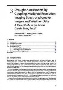
FIG. 1. Location of the study area. (a) Arkansas–Red River basin 1-km topographic data and watershed boundaries of 144 interior USGS hydrologic units (HUC). (b) Baron Fork at Eldon (808 km2), Baron Fork at Dutch Mills (107 km2), and Peacheater Creek (64 km2) topographic representation in the tRIBS model including modeled stream network, discharge gauging stations, and outlines of NEXRAD 4-km radar grid cells.

tions and potential radar errors over this region, with consequent effects for hydrologic applications (Smith et al. 1996; Grassotti et al. 2003).

d. Hydrometeorological flood events Two storm periods in 1998 were selected for evaluating the combined rainfall and flood forecasts in the Baron Fork watershed. While the selection of only two events is limiting, the intent of this study is to quantify the flood forecasting skill for storms that exhibit largescale features. A third event during the spring season (April 1999) was considered, but the nowcasting skill was lower due to its lack of large-scale organization (Van Horne et al. 2003). Other criteria for event selection included 1) availability of complete radar data from a validation period (Grassotti et al. 2003), 2) significant flooding levels observed at multiple stream

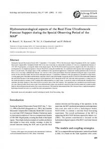
gauges, and 3) varying storm characteristics within an organized system. The two selected events exhibit linear, frontal organization (e.g., squall line) making them amenable to the nowcasting model as the large-scale storm envelope can be predicted reasonably well (Wolfson et al. 1999; Van Horne et al. 2003). Nevertheless, the storm characteristics were sufficiently different to illustrate the relative performance of the radar nowcasting and distributed flood forecasting models. Figure 2 presents the spatial distribution of the two storms during the peak rainfall period over the Baron Fork basin obtained from the WSI NOWrad product. The storms either caused flooding exceeding the regulatory limits set by the U.S. Army Corps of Engineers, Tulsa District, at BF (563.5 m3 s⫺1) and DM (283.4 m3 s⫺1) or constituted the annual peak flood (e.g., largest flood during the year) in one of the three gauges of interest.

FIG. 2. Regional distribution of instantaneous rainfall amount (mm h⫺1) during the peak storm period over Baron Fork obtained from WSI observations (4 km, 15 min). Note the location of the NEXRAD radar sites, marked with an “⫻” and three-letter site name, utilized in the radar composite. (a) 1300 UTC 4 Jan 1998 and (b) 1600 UTC 5 Oct 1998.

AUGUST 2006

665

VIVONI ET AL.

1) 4–8 JANUARY 1998 This hydrometeorological event was connected with a major intrusion of arctic air into the southern plains. Precipitation began as an unorganized event and then formed into a slow-moving frontal storm. Over the Baron Fork, this long-duration storm brought significant amounts of rainfall (Table 3). The storm moved from west to east oriented in a northeast to southwest direction. The rainfall spatial variability illustrates a gradient in accumulation with higher rainfall in the southeast corner (Fig. 3a). Basin response to the storm was pronounced, with 894, 492, and 62 m3 s⫺1 in peak discharge recorded at the BF, DM, and PC gauges, respectively (Fig. 4a). The flood response is of high magnitude in relation to historical floods with a 6.75-yr return period at BF (Fig. 5). The runoff ratio computed from observations is quite high (␾ ⫽ 1.2), suggesting contributions from high antecedent wetness and basin storage prior to the event. In addition, the basin lag time, computed as the difference between the centroid of the basin-averaged rainfall and the hydrograph peak, is relatively short (tB ⬃13 h), suggesting a quick runoff response due to prior wetness conditions and possible overland flow.

2) 5–6 OCTOBER 1998 As a linear, highly organized convective system, this event is characteristic of the fall storms in the region (e.g., Bradley and Smith 1994). The storm initially developed as several convective cells and grew into a continuous, intense squall line moving eastward and oriented northeast to southwest. During its 20-h duration, the rainfall intensity varied as the storm moved upstream along the main river axis of the Baron Fork (Fig. 3b). The high rainfall amounts over the northeast corner induced a variable response, resulting in a decaying flood wave downstream (Fig. 4b). For the Baron Fork, the flood peak represents a 1.43- and 2.26-yr return period at BF (274 m3 s⫺1) and DM (289 m3 s⫺1), respectively (Fig. 5). As compared to the January event, the flood had a longer lag time between the rainfall centroid and the peak discharge (tB ⬃15 h) and lower runoff ratio (␾ ⫽ 0.24), indicating a drier basin condition prior to the flood event. Table 3 presents further

comparison of the January and October events in terms of key storm and flood characteristics.

e. Model calibration and hydrologic response The tRIBS model was calibrated separately for each storm period (approximately one month) using the multiple-gauge observations at BF, DM, and PC and baseline simulations for the Baron Fork basin over a 7-yr period (1993–2000) reported by Ivanov et al. (2004b). Treating each event individually is justified based on the differences in flood response, in particular the runoff ratio and lag time. A nested calibration was followed where the parameters of each subbasin (e.g., soil, aquifer, and channel properties) were modified prior to calibrating the overall watershed response. Only minor modifications were made to the baseline calibrations to ensure appropriate performance at the three gauging sites. Note that the individual calibration periods reduce the model uncertainty with respect to observations when comparing the QPF-based flood forecasts to the QPE-based flood hindcasts. In this experimental design, validation of the flood forecast for periods outside the two events is not considered [see Ivanov et al. (2004a,b) for model validation results]. Initial parameter estimates were based on physical relations to soils and vegetation properties and their spatial distributions. The initial water table distribution was obtained using an algorithm relating the topographic distribution to the initial baseflow condition following Sivapalan et al. (1987). Ivanov et al. (2004a,b) present further details on the model calibration and initialization strategy, including parameter definitions, sensitivity, and optimized values for the study basin. To further reduce initialization errors, a dry spinup period of several weeks was allowed before each flood event simulation following Vivoni et al. (2005). Note that the low streamflow conditions (Fig. 4) prior to each flood allow for this initialization strategy. Figure 6 presents the calibrated tRIBS model streamflow response to WSI radar rainfall data (4 km, 15 min) for the two flood events at the three gauging stations. In addition, Table 4 presents several goodness-of-fit statistics that quantify the calibrated model performance relative to the observed hydrographs (see section 3c for

TABLE 3. Storm characteristics for Baron Fork events. D is the rainfall duration (h); I15 is the maximum 15-min intensity at any radar cell (mm h⫺1); PT is the total basin-averaged rainfall (mm); RT is the total runoff (mm); ␾ is the runoff ratio (PT /RT); Qp is the observed peak discharge (m3 s⫺1); tB is the basin lag time (h); tR is the estimated return period (yr). Period

D (h)

I15 (mm h⫺1)

PT (mm)

RT (mm)

␾ (–)

Qp (m3 s⫺1)

tB (h)

tR (yr)

4–13 Jan 1998 5–8 Oct 1998

30.5 20.0

52.02 36.66

98.51 83.17

117.86 20.13

1.20 0.24

893.93 273.85

13.25 15.25

6.75 1.43

666

JOURNAL OF HYDROMETEOROLOGY

VOLUME 7

FIG. 3. Spatial distribution of normalized total rainfall for selected storm periods from WSI observations (4 km, 15 min). Normalization is performed with the maximum rainfall accumulation in the total rainfall field; value shown in parentheses. (a) January 1998 (163.27 mm) and (b) October 1998 (152.16 mm).

definitions). The simulated discharge is available at the model time step for the unsaturated zone dynamics (3.75 min in this study) and compared to hourly observations resampled to the same temporal resolution. In addition to rainfall data, surface meteorological observations at the hourly scale are used to drive the radiation and energy balance within the model (Maurer et al. 2002). As shown by a visual comparison of the multiplegauge hydrographs (Fig. 6) and the values of the statistical metrics (Table 4), the calibrated model adequately reproduces the flood events as compared to observations. Discrepancies in peak discharge and time to peak within the subbasins may be due to inaccuracies in the radar rainfall estimates, stream discharge observations, or calibration parameters. Overall, the multiple-gauge calibration provides confidence in the distributed hydrologic model as a numerical laboratory and its capability for streamflow prediction in the gauged basins.

Performance at the gauged sites is also sufficiently accurate to test the model capabilities in forecast mode at ungauged sites in the watershed, as described in Table 5. Note that comparisons at ungauged sites are performed to assess the catchment-scale dependence of the radar nowcasting technique relative to the calibrated hydrological model at those locations.

3. Rainfall and flood forecasting experiments The rainfall and flood forecasts generated from the STNM and tRIBS models are illustrated in a simulated real-time setting in two modes of operation, interpolation and extended-lead forecasting. Figure 7 presents a schematic of the methods for temporally combining the rainfall and flood forecasts. The two forecasting modes are designed to mimic the operational coupling of the two models in circumstances where the nowcasting

FIG. 4. Observed mean areal rainfall (top) for Baron Fork from the WSI product (mm h⫺1) and (bottom) USGS discharge observations (m3 s⫺1) for each gauged basin. (a) January 1998 and (b) October 1998. Note the horizontal lines in (a) are the U.S. Army Corps of Engineers regulatory flood limits at BF (long dash, 563.5 m3 s⫺1) and DM (short dash, 283.4 m3 s⫺1).

AUGUST 2006

VIVONI ET AL.

FIG. 5. Sample flood frequency distribution (probability of nonexceedance) based on annual peak observations from 1945 to 2001 (BF) and 1958 to 2001 (DM). The open symbols represent the flood events considered in this study. The horizontal lines represent the U.S. Army Corps of Engineers regulatory flood limits at BF (dashed, 563.5 m3 s⫺1) and DM (dashed–dot, 283.4 m3 s⫺1).

products (a) can be used to fill in missing radar data (interpolation) or (b) can be used to generate a forecasted rainfall sequence at single lead time (extendedlead forecasting). In an operational setting, rainfall forecasts of increasing forecast lead time as produced by the interpolation mode would be used to drive the hydrological model. Extended-lead forecasting is similar to a hindcast experiment except that during the forecast interval QPEs are replaced with QPFs of the same lead time. This isolates the effect of lead time on the quality of the rainfall forecast for use in a flood forecast. Since our experiments are in a simulated real-time setting, our objective is to identify the sensitivity of the flood forecast skill as a function of lead time, basin size, and rainfall variability for each STNM forecast mode. In the following, we describe each operational mode designed to examine the hydrologic response to various rainfall specifications.

a. Interpolation mode In the interpolation mode experiments, we utilize the nowcasting capabilities of the STNM model to extrapolate rainfall fields between available radar images, an operation that fills in missing data (e.g., an interpolation). The rainfall forcing to the tRIBS hydrologic model is the radar-based QPEs for time periods of data availability and the STNM-based nowcasting rainfall fields for the hydrologic model time steps during which radar data are unavailable. Typically, QPEs can be minutes to hours apart in an operational setting where scan

667

intervals and data processing may impose practical limits on the sampling interval. The interpolation mode can be useful in operational forecasting as missing rainfall observations are filled in by forecasts of varying lead time based on the short-term advection of available QPEs. For comparison, a persistence forecast is generated by replacing the rainfall forecasts with the last available QPE during periods of missing rainfall observations. In Fig. 7a, the interpolation mode is illustrated over a simulation period defined by a start (TS) and final time (TF). Rainfall forecasts from STNM or persistence begin at TI and lasts for a period defined by the lead time (tL). Prior to TI, tRIBS is forced with QPEs. Rainfall forecasts using available QPEs up to and including TI are used for the interval TI ⬍ t ⱕ TI ⫹ tL during ⌬T steps. This procedure is repeated for the next available QPE until TF. During the flood forecast interval (TI to TF), a sequence of variable-length rainfall forecasts is constructed for each tL time interval based on all previous QPEs. For example, in Fig. 7a the lead time is tL ⫽ 3⌬T and a single rainfall forecast interval is composed of the radar QPE and ⌬T, 2⌬T, and 3⌬T QPFs. For this study, ⌬T is selected as the temporal resolution of the radar data (15 min), while tL is varied from 15 min to 3 h. The resulting QPFs are a temporal interpolation of the radar QPEs using a mixture of rainfall forecasts of variable lengths and skill until the lead time (tL) is reached.

b. Extended-lead forecast mode In the extended-lead forecast mode, we use radar rainfall nowcasting to extend the lead time of the hydrologic forecasts due to improved knowledge of future rainfall, thus eliminating the negligible precipitation assumption. The rainfall forcing to the tRIBS model is composed of a sequence of QPFs of equal lead time (tL) produced from a continuously available set of QPEs. Without the extended-lead QPFs, the rainfall forcing terminates at the current time and flood forecast skill decays rapidly in the subsequent period. This technique utilizes the STNM model to provide a series of fixedlength rainfall forecasts that are appropriate when the radar temporal resolution is high. The advantage of this mode is that the hydrologic lead time is extended by the lead time of the nowcast. Use of the extended-lead forecast mode is preferable when the available radar products have a high temporal resolution and an increase in forecast lead time is sought. In Fig. 7b, the extended-lead forecast mode is shown over the simulation interval (TS to TF). Rainfall forecasts from the STNM model are generated at a selected tL for all available QPEs. The tRIBS model is forced

668

JOURNAL OF HYDROMETEOROLOGY

VOLUME 7

FIG. 6. Comparison of observed and simulated hydrographs (m3 s⫺1) from the calibrated tRIBS model for the two flood events: (left) January 1998, (right) October 1998, and three gauges: (top) BF, (middle) DM, and (bottom) PC. See Table 4 for goodness-of-fit statistics between the observed and simulated hydrographs.

with fixed-lead-time QPFs beginning at TI over the flood forecast interval (TI to TF) in ⌬T steps. For example, in Fig. 7b the lead time is tL ⫽ 3⌬T and a forecast interval is composed of QPFs of fixed lead time 3⌬T. In this study, ⌬T is selected as the radar temporal resolution (15 min), while tL is varied from 15 min to 3 h. The resulting QPFs are a series of equivalent leadtime nowcasts generated from different radar QPEs such that the rainfall forecast skill is identical and highly dependent on the selection of the forecast lead

time (tL). Note that the interpolation mode is a mixture of QPFs of sequential forecast lead times, while the extended-lead forecast mode is a collection of rainfall forecasts of equal or fixed lead time.

c. Performance metrics Model performance for the two operational modes is assessed using four metrics to compare discharge observations (O) and forecasts (F ): correlation coefficient

AUGUST 2006

669

VIVONI ET AL.

TABLE 4. Calibrated model performance for the two flood events at the three gauging stations (BF, DM, and PC). E is the efficiency (⫺); CC is the correlation coefficient (⫺); B is the bias (⫺); MAE is the mean absolute error (m3 s⫺1). Comparisons are made between the observed USGS discharge and the calibrated model simulation as shown in Fig. 6. See Eqs. (1)–(4) for details on the derivation of each skill metric.

Period and basin 4–8 Jan 1998 BF DM PC 5–6 Oct 1998 BF DM PC

E (⫺)

CC (⫺)

B (⫺)

MAE (m3 s⫺1)

0.84 0.78 0.76

0.95 0.92 0.92

0.68 0.72 0.76

42.03 9.10 2.57

0.69 0.78 0.73

0.87 0.91 0.90

1.29 1.61 1.32

14.40 5.93 0.31

(CC), efficiency coefficient (E ), bias (B), and mean absolute error (MAE). The correlation coefficient is

FIG. 7. Schematic of the coupling between the rainfall and flood forecasting models with forecast lead time tL ⫽ 3⌬T, as an example. Rainfall inputs to the hydrologic model are gridded fields (radar QPEs or STNM QPFs) available at regular time intervals (⌬T ) over the simulation period TS ⱕ t ⱕ TF. (a) Interpolation mode and (b) extended-lead forecast mode. Note the interpolation mode utilizes a sequence of variable-length forecasts (e.g., QPE, ⌬T, 2⌬T, 3⌬T QPFs) after QPE availability, while the extended-lead forecast mode uses a sequence of fixed-length forecasts (e.g., 3⌬T QPFs) derived from available QPEs.

N

兺 共O ⫺ O兲共F ⫺ F兲 i

CC ⫽

冋兺

i⫽1

N

i

册 冋兺 0.5

共Oi ⫺ O兲2

i⫽1

N

册

0.5

共Fi ⫺ F兲2

i⫽1

,

共1兲

where the overbar denotes a mean value, and CC measures the linear relation between F and O. Here CC varies from ⫺1 (negative) to 1 (positive) with CC ⫽ 0 indicating no correlation. Each summation is over the total number (N ) of time periods in the observed and TABLE 5. Subbasin characteristics at gauged and ungauged forecast points. A is the basin area (km2); L is the maximum distance to the subbasin outlet (km); S is the relief ratio (m km⫺1); Dd is the drainage density (km⫺1); tc is the time of concentration (h) ⫺0.385 , where units are L from Kiprich (1940): tc ⫽ 0.000325 L0.77 S (m) and S (m m⫺1).

Basin

A (km2)

L (km)

S (m km⫺1)

Dd (km⫺1)

tc (h)

1 2 3 4 5 (PC) 6 7 8 9 10 (DM) 11 12 13 14 15 (BF)

108.23 1.41 2.67 12.14 65.06 610.60 450.26 365.25 182.91 106.91 49.07 21.18 4.29 0.78 808.39

25.73 2.59 4.52 8.06 19.90 50.33 40.01 35.03 29.78 18.64 12.72 9.03 3.53 1.33 67.26

6.06 34.01 21.44 14.94 9.26 6.81 8.11 9.09 9.49 13.41 19.10 24.92 51.27 112.77 5.47

0.9895 0.8264 0.7701 0.8059 0.8293 0.8355 0.8352 0.8209 0.8230 0.8370 0.8692 0.8700 0.7720 0.3033 0.8630

5.78 0.51 0.93 1.67 4.03 9.26 7.25 6.27 5.44 3.32 2.16 1.50 0.55 0.19 12.59

forecasted discharge records. The efficiency (E ) improves upon CC for model evaluation (Legates and McCabe 1999): N

兺 共O ⫺ F 兲

2

i

E⫽1⫺

i

i⫽1

,

N

兺 共O ⫺ O兲

共2兲

2

i

i⫽1

where E varies from –⬁ to 1, with larger values indicating improvements and E ⱕ 0 implying the observed mean is as good as or better than the model forecasts. The dimensionless bias (B) measures the correspondence between the mean observations and forecasts: B⫽

F O

共3兲

,

defined following Grecu and Krajewski (2000). The MAE (m3 s⫺1) describes the absolute difference between the observations and forecasts without emphasizing the value of outliers (Legates and McCabe 1999): MAE ⫽

1 N

N

兺 | O ⫺ F |. i

i

共4兲

i⫽1

We assess model performance by comparing forecasts with QPE-driven flood predictions (or hindcasts) taken as a ground truth (i.e., observations, O). Furthermore, the skill metrics are used to determine flood predictability as function of spatial and temporal scale.

670

JOURNAL OF HYDROMETEOROLOGY

VOLUME 7

FIG. 8. Flood forecast skill as a function of forecast lead time (tL in h) for the two selected storm events in BF using the interpolation mode to combine the STNM and tRIBS models: (a) efficiency, (b) correlation coefficient, (c) bias, and (d) mean absolute error. Each point is the time series statistic measuring the “goodness of fit” between a QPE-driven simulation (Fig. 6) and QPF-based flood forecast. Line segments between different lead times are drawn only for visualization purposes.

4. Results In the following, we summarize the combined forecasting experiments over the Arkansas–Red River basin (STNM model) and Baron Fork watershed (tRIBS model) for the two selected events (January and October 1998). A significant number of calibrated tRIBS model runs were performed using the various forecasting modes. Results are presented via comparisons between the QPE-driven and QPF-driven model hydrograph responses at multiple gauging stations. Here, we focus on the flood forecast performance as a function of rainfall forecast lead time, basin scale, and rainfall spatial distribution for the interpolation and extended-lead forecast modes. Note that the sample size in our experiments is small, given the limited number of storm events and selected metrics. For brevity, we present the results for the interpolation mode, although conclusions are derived based on the inspection of the results of both forecasting techniques. In addition, we present a comparison between the two modes and a

persistence forecast and present a method for quantifying the space–time predictability of floods using a combination of radar nowcasting and distributed hydrologic modeling.

a. Temporal and spatial dependence of multiple-gauge flood forecasts 1) FORECAST

LEAD-TIME DEPENDENCE

The dependence of rainfall forecast skill on the lead time since the last available observation has been well documented (e.g., Georgakakos 1986; Pereira Fo et al. 1999; Grecu and Krajewski 2000) and is expected as advection-based forecasts are incapable of generating new features of the precipitation field. Van Horne et al. (2003) quantified the decrease in forecast skill of the STNM nowcasting model for the January and October 1998 events through the use of the critical success index (CSI) over the Arkansas–Red River basin. As lead time was increased from 0.25 to 2 h, the CSI performance of

AUGUST 2006

671

VIVONI ET AL.

FIG. 9. Flood forecast skill as a function of basin area (A in km2) for the two selected storm events using the interpolation mode at the 1-h forecast lead time: (a) efficiency, (b) correlation coefficient, (c) bias, (d) and mean absolute error.

the WSI-based STNM forecast decreased in comparison to the observed radar fields. The decrease in rainfall predictability with lead time should translate to a reduction in flood forecast skill in the combined STNM–tRIBS models. To test this, model runs in the interpolation and extended-lead forecast modes were evaluated as a function of lead time (e.g., 12 lead times, at 15-min spacing, for each storm and mode). Figure 8 presents the lead-time variation of E, CC, B, and MAE for the two storm events using the interpolation mode. These metrics compare the forecast hydrograph to the QPE-driven simulation at the basin outlet. Note the marked decrease in skill (E and CC decrease; B and MAE increase) as tL is increased beyond 1 h for the October storm, but a slower decrease in skill for the January event. In some cases, forecast skill varies nonmonotonically due to the effects of interpolating QPEs providing varying amounts of information to the advection forecast as lead time is increased. In addition, note a reversal in the relative skill at tL ⫽ 1 h between the two storms, suggesting more

dynamical changes for the October event. The general decrease in forecast skill with tL indicates the effect of the temporal spacing between available QPEs. These results suggest that the rainfall lead time limits flood forecast skill. Similar results were found for the extendedlead forecast mode (see Fig. 11), although a smoother variation with lead time is apparent. In general, the performance of the combined rainfall–flood forecasts is observed to be both lead time and storm dependent.

2) CATCHMENT-SCALE

DEPENDENCE

The dependence of flood forecast skill on catchment scale has received much less attention, in part due to the inability of lumped models to predict hydrographs at internal gauges. Most rainfall–runoff studies focus on a particular watershed without considering the variability in response with basin scale (e.g., Mimikou and Baltas 1996; Pereira Fo et al. 1999; Yates et al. 2000; Dolciné et al. 2001). With the advent of weather radar data and distributed hydrologic models, it is now feasible to address scaling issues in the context of flood

672

JOURNAL OF HYDROMETEOROLOGY

forecasting. The scales that can be resolved with these tools range from the resolution of the radar data (e.g., pixel area of ⬃16 km2) up to the basin area feasibly simulated with a distributed model (e.g., 102 to 105 km2). A relation between catchment scale and forecast skill as a function of lead time would be useful forecasting knowledge. To test dependence on spatial scale, the forecast model runs were evaluated as a function of basin area. The interior basins (ungauged forecast points) in Table 5 represent a range of physiographic properties, including a difference in area (A) of three orders of magnitude (⬃0.8 to 800 km2). For the interpolation mode at a lead time of 1 h, Fig. 9 presents the variation of flood forecast skill (E, CC, B, and MAE) with basin area for both events. We selected the 1-h lead time due to the high skill determined during prior experiments. Note the improvement in flood forecast skill as A is increased beyond 200 km2 for both storms. For smaller areas, values of E, CC, and B vary considerably and can be quite low at the 1-h lead time. This is primarily due to the forecast errors introduced for small basins covered by a single radar pixel (⬃16 km2). Both E and CC stabilize to values greater than 0.9 for basin areas A ⱖ 200 km2, while B fluctuates around unity after A ⬃200 km2. The MAE behaves differently as it can increase or decrease with basin area. Similar results were obtained for the extended-lead forecast mode at 1-h lead times. In general, the metrics (E, CC, and B) show a spatial dependence in the forecast skill with an identified threshold beyond which performance is similar. Note also that forecast skill for January is superior to the October event except for the largest basin scales (reduced E and CC, and increased B and MAE), suggesting greater-scale improvements for the latter storm due to the characteristics of the flood event (e.g., progressive decreases in the flood discharge with basin area for the October event; see Fig. 4).

3) RAINFALL

SPATIAL VARIABILITY DEPENDENCE

Flood event predictability depends on the nowcasting ability to accurately forecast rainfall amounts in the appropriate place and time (Collier and Krzysztofowicz 2000). In describing the space–time forecast dependence, the combined STNM–tRIBS models have utilized the full radar spatial content and the spatial sensitivity of the hydrologic model. Therefore, forecast skill can be further investigated by separating the effects of the spatial distribution from the temporal variation of the rainfall forecast. This is frequently done for assessing the impact of rainfall variability on hydrologic simulations (e.g., Pessoa et al. 1993; Shah et al. 1996; Bell and Moore 2000).

VOLUME 7

FIG. 10. Impact of spatial rainfall structure on the flood forecast skill for the interpolation mode stratified by lead time (0–1, 1–2, and 2–3 h). Symbols above the 1:1 line (CCMAP vs CCDistributed) imply improved flood forecast skill for the MAP-based rainfall forecast as compared to the distributed radar QPFs. Each symbol represents an individual subbasin (15 total) for a particular lead time (12 different tL over 3-h period at 15-min resolution) and for each storm event. Both January and October 1998 events considered.

To test the importance of the rainfall spatial variation, we compare the forecasts using the interpolation mode and the fully-distributed radar data, with a mean areal precipitation (MAP)-based forecast derived from the original QPF field. The basin-averaged rainfall is identical in its temporal variation to the STNM forecast, but consists of a uniform forecast value for the entire basin. As a result, the MAP-based forecast rainfall loses its spatial structure but retains its lead-time dependence. Figure 10 compares the relative skill of the distributed (CCDistributed) and MAP (CCMAP) forecasts. Each symbol represents a different subbasin for each storm event at a particular lead time. The results are stratified into three lead-time categories: 0–1, 1–2, and 2–3 h. This classification shows that for low tL (0–2 h), forecast skill is greater for the distributed rainfall (higher CC). For high tL (⬎2 h), the MAP forecast outperforms the distributed QPF product. This suggests that retaining the rainfall spatial variability is most important for short tL while a basin-averaged product may be advantageous for larger lead times. The result is an indication that the correct spatial structure in the nowcast product is often lost after a particular lead time.

b. Quantitative comparisons of rainfall–flood forecast modes The flood forecast skill for the operational modes is compared to a persistence forecast for the two storm

AUGUST 2006

VIVONI ET AL.

673

FIG. 11. Flood forecast skill vs lead time for the (left) January 1998 and (right) October 1998 storm events at the (top) ungauged subbasin 12 (21 km2), (middle) DM (107 km2), and (bottom) BF (808 km2). Three forecasts modes are compared for each storm event, subbasin area, and forecast lead time (interpolation mode, extended-lead forecast mode, and persistence). Line segments between different lead times are drawn only for visualization purposes.

events and in three nested basins (Fig. 11). Persistence assumes a static rainfall field after a particular QPE is available over the lead time (tL) while the STNM nowcasts can mimic storm dynamics. Although there is considerable variability in the forecast performances, we can elucidate some key features. The persisted rainfall provides the highest forecast skill for short lead times (tL ⱕ 0.75 h) across basin scales and storm events since the STNM may introduce errors not present in the persisted forecast. For short lead times, high persistence skill is due to adequate provision of rainfall amounts during periods of minor changes. Storm evolution over a basin determines the lead time over which persistence has a higher forecast skill relative to the other modes. Note the nowcasting product is designed to advect large-scale features at the expense of embedded cells, retained in the persistence forecast. When regional rainfall patterns change quickly, a persistence forecast

will likely underperform relative to the STNM QPFs. For example, persistence has lower skill for tL ⱖ 1 h in the ungauged subbasin for the January event. Capturing storm dynamics through nowcasting is critical for lead times in the range of 1–3 h. In a similar study, Dolciné et al. (2001) found that nowcasting was superior to persistence in terms of rainfall-flood forecast skill. Flood forecast skill varies between the interpolation and extended-lead forecast modes with the particular storm dynamics. In addition to varying smoothly with tL, the extended-lead forecast mode tends to perform better in events exhibiting growth, decay, or rapid motion (October). For storms that retain their structure as they pass over the basin (January), the interpolation mode forecast is superior. These differences are related to the formulation of each mode. Using nowcasting to fill in missing data (interpolation) benefits from slow

674

JOURNAL OF HYDROMETEOROLOGY

FIG. 12. Space–time scale dependence of the flood forecast skill, measured by the correlation coefficient (CC), for the smallest seven ungauged subbasins during the two flood events. Note that the interpolation mode lead time (tL) is normalized by the time of concentration (tc) for each subbasin (see Table 5). The range of basin sizes (0.78 to 49.07 km2) is comparable to the minimum resolution of a radar cell (16 km2).

changes in storm structure, while storm growth and decay is explicitly retained in fixed-length (extended lead) forecasts that consider all available data. A comparison of the overall performance for each event suggests the two modes exhibit similar trends in forecast skill with lead time and basin scale.

c. Effects of scale on rainfall–flood forecast skill Identifying the space–time scales over which the combined forecasts have high skill is critical for determining flood predictability. Using the nowcasting model, flood forecast skill has been shown to decrease with lead time for one basin scale (Fig. 8) and increase with basin area at a single lead time (Fig. 9). A useful synthesis of both effects can be derived by scaling the forecast lead time with the basin time of concentration (tc). Table 5 presents tc for each Baron Fork subbasin, computed from the relief ratio (S) and length (L) in the subbasin (Kirpich 1940). As an empirical estimate of the basin response time, tc provides a means for scaling tL without knowledge of the storm-dependent response in each subbasin. In this context, tc captures differences in basin spatial scale. Figure 12 shows the variation of flood forecast skill, quantified by the correlation coefficient (CC), with respect to the space–time scale (tL /tc) for the interpolation mode. The results are limited to the smallest subbasins (A ⫽ 0.78 to 49.07 km2) since these watersheds have response times (tc ⫽ 0.19 to 2.16 h) within the

VOLUME 7

maximum forecast lead time (tL ⫽ 3 h). Note that flood forecast skill decreases sharply for values of tL /tc ⬎ 1, suggesting that the limit of flood predictability is related to this scale. For rainfall forecast with tL less than the basin response time, the flood forecast skill is high. As the forecast lead time increases relative to the basin spatial scale (tc), flood forecast skill deteriorates significantly. This suggests that nowcasting predictions work best within basins whose response time is on the order or less than the rainfall forecast lead time as the dynamics of the storm event within the basin can be captured reliably by the extrapolation method. Using the normalized space–time scale tL /tc for different events and forecasting models may serve as an adequate indication of rainfall–flood predictability. The general nature of tL /tc as a limit of predictability should be verified through the combined use of radar nowcasting and distributed flood forecasting tools in other storm events and basins.

5. Discussion and conclusions The primary objective for utilizing rainfall forecasts in hydrologic models is to increase the flood and flash flood warning time and forecast accuracy by eliminating the assumption of negligible future rainfall during storm development. In this study, an algorithm based on the extrapolation of large-scale storm motion is used to derive short-term, radar-based rainfall predictions for two organized frontal events over Oklahoma. Rainfall forecasts from the nowcasting algorithm are subsequently used in a distributed hydrologic model to produce multiple-gauge flood forecasts. Through comparisons to radar-driven simulations, the flood predictability of the combined models is assessed in a simulated real-time operation using two different modes: interpolation and extended-lead forecasting. Results from the study indicate the following: 1) Flood prediction skill decreases with forecast lead time over the entire watershed and in selected subbasins for the two storm events considered. The decrease in forecast skill is related to the characteristics of each storm (e.g., translation, growth, and decay) and can vary for the two operational forecast modes. Both modes provide superior performance as compared to a persistence forecast for lead times greater than 1 h. 2) Flood forecast skill increases with catchment area over a selected forecast lead time (1 h) for the two storm events considered. The increase in forecast skill is related to the reduction of nowcasting errors as basin scale is increased and varies for each storm

AUGUST 2006

VIVONI ET AL.

due to the characteristics of the flood event (e.g., downstream flood propagation). 3) Distributed flood forecast skill improves for short lead times (0 to 2 h) when the spatial structure of a radar nowcast is retained. For longer lead times (2 to 3 h), a basin-averaged rainfall forecast demonstrates higher skill, consistent with the increased uncertainty on the spatial variability in the nowcasting product as lead time increases. 4) The rainfall–flood forecast performance is shown to be a function of the ratio of the rainfall forecast lead time to the basin time of concentration (tL/tc), a normalized space–time scale. Forecast skill decreases for tL/tc ⬎ 1, implying that nowcasting forecasts deteriorate for basins whose response time is shorter than the forecast lead time. The results of this study are based on two storms exhibiting organized, large-scale features making them amenable to radar nowcasting via a scale-separation technique (e.g., Wolfson et al. 1999; Van Horne et al. 2003). The two linear storms produced flooding in a set of nested watersheds in Oklahoma whose characteristics are representative of the southern plains (Ivanov et al. 2004b; Reed et al. 2004). While the selection of two storm events in a regional watershed is somewhat limiting, we believe that the results discussed above are indicative of the hydrometeorological predictability that can be achieved using combined radar nowcasting and distributed flood forecasting. In particular, we have focused on utilizing the strengths of the distributed approach to identify the potential relation between catchment scale and flood forecast skill as a function of lead time. A space–time scale based on the ratio of the forecast lead time and the basin response time (tL/tc) is shown to clearly identify a significant decrease in rainfall–flood predictability for the two events considered in this study. The general nature of this result for other storm settings and watershed characteristics requires further investigation. Nevertheless, this set of analysis suggests that hydrometeorological forecast skill using radar nowcasts is high for the space–time scales corresponding to flood events in small, headwater basins where the lead time of the rainfall forecast is less than the basin response time. This result is particularly encouraging as the predictability of flash flood events is considered a difficult problem in research and operational hydrometeorology. As basin size increases, the flood forecasting problem shifts from uncertain knowledge of rainfall input to the more predictable estimation of flood propagation (Garrote and Bras 1995). The combined forecast system takes advantage of a high-resolution, operational radar network. For gener-

675

ating flood predictions utilizing all available radar data, two techniques were developed to provide variablelength (interpolation mode) or fixed-length (extendedlead forecast mode) flood forecasts. The two modes can improve the flood forecast skill in relation to a persistence forecast, in particular over 1–3-h lead times. Quantifying flood forecast skill with respect to lead time, basin scale, and rainfall spatial variability is of primary importance for any hydrometeorological forecasting system, yet there have been few attempts of quantitative verification (e.g., Georgakakos 1986; Pereira Fo et al. 1999; Dolciné et al. 2001) as performed in this study. To further extend long-lead forecast skill, rainfall forecasts from atmospheric models and satellite rainfall nowcasting should be evaluated within the existing framework (e.g., Grassotti et al. 2002; Ganguly and Bras 2003). In particular, predictions from meteorological models could provide skill over longer lead times. A promising development is the lead-timedependent fusion of rainfall forecasts from multiple model sources as conceptualized by Browning and Collier (1989) and Collier (1991). Distributed hydrologic models provide new opportunities for flood forecasting in multiple, nested basins of varying scale. Despite advantages of the distributed approach, there are few studies that have addressed the flood forecast improvements due to radar nowcasting (Mecklenburg et al. 2000; Berenguer et al. 2005). Flood prediction in interior catchments provides information on the differential runoff production within a basin and its propagation through the channel network as a function of rainfall spatial variability. In an operational setting, the spatiotemporal variation of flood discharge may improve existing flood warning techniques. Whereas lumped models treat a basin as a single unit, distributed models consider variations in rainfall, topography, and surface properties. Furthermore, distributed models provide quantitative predictions of internal hydrologic states and fluxes, which may be useful in many applications but are unattainable with lumped operational models. Understanding the space–time predictability of soil moisture, for example, is a promising area of research that can also be addressed with the combined use of a radar nowcasting and distributed hydrologic models. Acknowledgments. This research was sponsored by the U.S. Army Research Office (Contract DAAD1900-C-0114) and NOAA (Contract NA97WH0033). We thank MIT Lincoln Laboratory for the use of the STNM nowcasting model and Weather Services International (WSI) for the radar rainfall data used in this study. We appreciate the comments from David N.

676

JOURNAL OF HYDROMETEOROLOGY

Yates (NCAR) and three anonymous reviewers that improved the original manuscript. REFERENCES ASCE Task Committee, 1999: Geographic information system modules and distributed models of the watershed. ASCE, Reston, VA, 120 pp. Bell, V. A., and R. J. Moore, 2000: The sensitivity of catchment runoff models to rainfall data at different spatial scales. Hydrol. Earth Syst. Sci., 4, 653–667. Benoit, R., P. Pellerin, N. Kouwen, H. Ritchie, N. Donaldson, P. Joe, and E. D. Soulis, 2000: Toward the use of coupled atmospheric and hydrologic models at regional scales. Mon. Wea. Rev., 128, 1681–1705. Berenguer, M., C. Corral, R. Sanchéz-Diezma, and D. SempereTorres, 2005: Hydrological validation of a radar-based nowcasting technique. J. Hydrometeor., 6, 532–548. Bradley, A. A., and J. A. Smith, 1994: The hydrometeorological environment of extreme rainstorms in the Southern Plains of the United States. J. Appl. Meteor., 33, 1418–1431. Browning, K. A., and C. G. Collier, 1989: Nowcasting of precipitation systems. Rev. Geophys., 27, 345–370. Carpenter, T. M., K. P. Georgakakos, and J. A. Sperfslagea, 2001: On the parametric and NEXRAD-radar sensitivities of a distributed hydrologic model suitable for operational use. J. Hydrol., 253, 169–193. Collier, C. G., 1991: The combined use of weather radar and mesoscale numerical model data for short-period rainfall forecasting. Hydrological Application of Weather Radar, I. D. Cluckie and C. G. Collier, Eds., E. Horwood, 331–348. ——, and R. Krzysztofowicz, 2000: Quantitative precipitation forecasting. J. Hydrol., 239, 1–2. Dixon, M., and G. Weiner, 1993: TITAN: Thunderstorm identification, tracking, analysis and nowcasting—A radar-based methodology. J. Atmos. Oceanic Technol., 10, 785–797. Dolciné, L., H. Andriue, D. Sempere-Torres, and D. Creutin, 2001: Flash flood forecasting with coupled precipitation model in mountainous Mediterranean basin. J. Hydrol. Eng., 6, 1–10. Droegemeier, K. K., and Coauthors, 2000: Hydrological aspects of weather prediction and flood warning: Report of the Ninth Prospectus Development Team of the U.S. Weather Research Program. Bull. Amer. Meteor. Soc., 81, 2665–2680. Dupree, W. J., M. M. Wolfson, R. Johnson, K. E. Theriault, B. E. Forman, R. A. Boldi, and C. Wilson, 2002: Forecasting convective weather using multi-scale detectors and weather classification. Preprints, 10th Conf. on Aviation, Range, Aerospace Meteorology, Portland, OR, Amer. Meteor. Soc., CDROM, 5.5. Ganguly, A. R., and R. L. Bras, 2003: Distributed quantitative precipitation forecasting using information from radar and numerical weather prediction models. J. Hydrometeor., 4, 1168–1180. Garrote, L., and R. L. Bras, 1995: A distributed model for realtime flood forecasting using digital elevation models. J. Hydrol., 167, 279–306. Georgakakos, K. P., 1986: A generalized stochastic hydrometeorological model for flood and flash-flood forecasting. 2. Case studies. Water Resour. Res., 22, 2096–2106. Golding, B. W., 1998: Nimrod: A system for generating automated very short range forecasts. Meteor. Appl., 5, 1–16. Gourley, J. J., and B. E. Vieux, 2005: A method for evaluating the

VOLUME 7

accuracy of quantitative precipitation estimates from a hydrologic modeling perspective. J. Hydrometeor., 6, 115–133. Grassotti, C., R. N. Hoffman, E. R. Vivoni, D. Entekhabi, V. Y. Ivanov, and M. P. Van Horne, 2002: Real-time hydrometeorological forecasting from radar and satellite observations. Final Rep., ARO DAAD-19-00-C-0114, 85 pp. ——, ——, ——, and ——, 2003: Multiple timescale intercomparison of two radar products and rain gauge observations over the Arkansas–Red River basin. Wea. Forecasting, 18, 1207– 1229. Grecu, M., and W. F. Krajewski, 2000: A large-sample investigation of statistical procedures for radar-based short-term quantitative precipitation forecasting. J. Hydrol., 239, 69–84. Hamill, T. M., and T. Nehrkorn, 1993: A short-term cloud forecast scheme using cross correlations. Wea. Forecasting, 8, 401–411. Ivanov, V. Y., E. R. Vivoni, R. L. Bras, and D. Entekhabi, 2004a: Catchment hydrologic response with a fully-distributed triangulated irregular network model. Water Resour. Res., 40, W11102, doi:10.1029/2004WR003218. ——, ——, ——, and ——, 2004b: Preserving high-resolution surface and rainfall data in operational-scale basin hydrology: A fully-distributed physically-based approach. J. Hydrol., 298, 80–111. Johnson, D., M. Smith, V. Koren, and B. Finnerty, 1997: Comparing mean areal precipitation estimates from NEXRAD and rain gauge networks. J. Hydrol. Eng., 4, 117–124. Kirpich, Z. P., 1940: Time of concentration of small agricultural watersheds. Civ. Eng., 10, 362. Kumler, M. P., 1994: An intensive comparison of triangulated irregular networks (TINs) and digital elevation models (DEMs). Cartographica, 31 (2), 1–48. Legates, D. R., and G. J. McCabe, 1999: Evaluating the use of “goodness-of-fit” measures in hydrologic and hydroclimatic model validation. Water Resour. Res., 35, 233–241. Maurer, E. P., A. W. Wood, J. C. Adam, D. P. Lettenmaier, and B. Njissen, 2002: A long-term hydrologically-based data set of land surface fluxes and states for the conterminous United States. J. Climate, 15, 3237–3251. McEnery, J., J. Ingram, Q. Duan, T. Adams, and L. Anderson, 2005: NOAA’s Advanced Hydrologic Prediction Service. Bull. Amer. Meteor. Soc., 86, 375–385. Mecklenburg, S., V. A. Bell, R. J. Moore, and J. Joss, 2000: Interfacing an enhanced radar echo tracking algorithm with a rainfall-runoff model for real-time flood forecasting. Phys. Chem. Earth B, 25, 1329–1333. Mimikou, M. A., and E. A. Baltas, 1996: Flood forecasting based on radar rainfall measurements. J. Water Resour. Plan. Manage., 122, 151–156. Moore, R. J., V. A. Bell, and D. A. Jones, 2005: Forecasting for flood warning. C. R. Geosci., 337, 203–217. Pereira Fo, A. J., K. C. Crawford, and D. J. Stensrud, 1999: Mesoscale precipitation fields. Part II: Hydrometeorologic modeling. J. Appl. Meteor., 38, 102–125. Pessoa, M. L., R. L. Bras, and E. R. Williams, 1993: Use of weather radar for flood forecasting in the Sieve basin: A sensitivity analysis. J. Appl. Meteor., 32, 462–475. Reed, S. M., and D. R. Maidment, 1999: Coordinate transformations for using NEXRAD data in GIS-based hydrologic modeling. J. Hydrol. Eng., 4 (2), 174–182. Reed, S., V. Koren, M. Smith, Z. Zhang, F. Moreda, D.-J. Seo, and D. M. I. P. Participants, 2004: Overall distributed model intercomparison project results. J. Hydrol., 298, 27–60.

AUGUST 2006

VIVONI ET AL.

Shah, S. M. S., P. E. O’Connell, and J. R. M. Hoskings, 1996: Modeling the effects of spatial variability in rainfall on catchment response. 2. Experiments with distributed and lumped models. J. Hydrol., 175, 89–111. Singh, V. P., and D. A. Woolhiser, 2002: Mathematical modeling of watershed hydrology. J. Hydrol. Eng., 7, 270–292. Sivapalan, M. K., E. F. Wood, and K. J. Beven, 1987: On hydrologic similarity: 2. A scaled model of storm runoff production. Water Resour. Res., 23, 2266–2278. Smith, J. A., D.-J. Seo, M. L. Baeck, and M. D. Hudlow, 1996: An intercomparison study of NEXRAD precipitation estimates. Water Resour. Res., 32, 2035–2045. Smith, K. T., and G. L. Austin, 2000: Nowcasting precipitation—A proposal for a way forward. J. Hydrol., 239, 34–45. Tsanis, I. K., M. A. Gad, and N. T. Donaldson, 2002: A comparative analysis of rain-gauge and radar techniques for storm kinematics. Adv. Water Resour., 25, 305–316. Van Horne, M. P., E. R. Vivoni, D. Entekhabi, R. N. Hoffman, and C. Grassotti, 2003: Short term radar nowcasting for hydrologic applications over the Arkansas–Red River basin.

677

Preprints, 17th Conf. on Hydrology, Long Beach, CA, Amer. Meteor. Soc., CD-ROM, J4.3. Vivoni, E. R., V. Y. Ivanov, R. L. Bras, and D. Entekhabi, 2004: Generation of triangulated irregular networks based on hydrological similarity. J. Hydrol. Eng., 9, 288–302. ——, ——, ——, and ——, 2005: On the effects of triangulated terrain resolution on distributed hydrologic model response. Hydrol. Processes, 19, 2101–2122. Wolfson, M. M., B. E. Forman, R. G. Hallowell, and M. P. Moore, 1999: The growth and decay storm tracker. Preprints, Eighth Conf. on Aviation, Range, and Aerospace Meteorology, Dallas, TX, Amer. Meteor. Soc., 58–62. Yates, D. N., T. T. Warner, and G. H. Leavesley, 2000: Prediction of a flash flood in complex terrain. Part II: A comparison of flood discharge simulations using rainfall input from radar, a dynamic model and an automated algorithmic system. J. Appl. Meteor., 39, 815–825. Young, C. B., A. A. Bradley, W. F. Krajewski, A. Kruger, and M. L. Morrissey, 2000: Evaluating NEXRAD multisensor precipitation estimates for operational hydrologic forecasting. J. Hydrometeor., 1, 241–254.