Extensions to Backward Propagation of Variance for Statistical Modeling

mdt2010020036.3d

26/2/010

11:57

Page 36

Compact Variability Modeling for Nanometer CMOS Technology

Extensions to Backward Propagation of Variance for Statistical Modeling Colin C. McAndrew Freescale Semiconductor

Ivica Stevanovic´ ABB Corporate Research Center

Xin Li GlobalFoundries

Gennady Gildenblat Arizona State University

Editor’s note: Correlating the statistics of process parameters with the statistics of electrical performance is a vital task in statistical modeling. This article describes a more general form of the backward propagation of variance (BPV) method, a numerical technique for iteratively solving the statistics of process parameters from the statistics of electrical performance within the behavior of models encapsulated in SPICE. Frank Liu, IBM Austin Research Lab

STATISTICAL SIMULATION IS IMPORTANT for the design of high-yield circuits,1 and statistical simulation requires statistical models. Such models can be generated using numerical techniques such as principal component analysis or factor analysis.2,3 However, physical models have proven substantially more accurate and efficient than strictly numerical models for retargeting statistical models (both for mean shifts and variance shifts in a process), predicting statistical models for a process based on previous generations of that process, and capturing unexpected or anomalous behavior in statistical variations over bias or geometry. The backward propagation of variance (BPV) technique is a unified approach for physically based statistical modeling, for both global and local (mismatch) statistical variations.4,5 In this article, we present recent extensions and enhancements to the BPV technique. We show how the assumption of a linear dependence of electrical performance on process parameters can be relaxed, and that correlations between different electrical performances can be explicitly included in the procedure. We include measures of circuit performance as modeling targets, and

36



0740-7475/10/$26.00 c 2010 IEEE

show that overspecifying the electrical performances to be modeled can improve overall statistical-modeling accuracy.

Backward propagation of variance

With the BPV approach, we can formulate statistical models as a set of independent, normally distributed process parameters, expressed as p ¼ ( p1, p2,. . ., pNp ). These parameters control the variations seen in device electrical performance, e ¼ (e1, e2,. . ., eNe ) ¼ e(p), through the behavior encapsulated in the SPICE models used for device and circuit simulation. Some process parametersfor example, those with large variations, such as the current density of the nonideal component of base current for bipolar junction transistors (BJTs)are better represented as log-normal distributions. Such behavior can still be modeled using a normally distributed process parameter by multiplying the parameter’s nominal value by the exponential of a normally distributed statistical process parameter. Partial correlations between parameters of the same or different devices can be modeled by writing those parameters as functions of combinations of independent process parameters.6 For example, the channel length variations LP and LN of PMOS and NMOS devices are partially correlated because they depend on the critical dimension (CD) of the polysilicon, which can be taken to be the same for the two device types because the polysilicon etch step that controls this is common. They also

Copublished by the IEEE CS and the IEEE CASS

IEEE Design & Test of Computers

Authorized licensed use limited to: FREESCALE SEMICONDUCTOR. Downloaded on March 26,2010 at 12:29:37 EDT from IEEE Xplore. Restrictions apply.

mdt2010020036.3d

26/2/010

11:57

Page 37

depend, however, on the out-diffusions of the p+ and n+ source-drain regions, ODP and ODN, that can be considered to be independent between the device types. We can accurately model partial correlations between LP and LN using only independent parameters by considering CD, ODP, and ODN as the fundamental statistical process parameters, rather than direct variations in LP and LN, and by introducing the following mappings:6 DLP ¼ CD þ ODP

(1)

device or circuit performance, and it does not distinguish between whether the electrical performance depends on process parameters from a single device type or from more than one device type. Nonetheless, in practice the BPV process has been applied to measures of device performance from only a single type of device. BPV verification based on a combination of device- and circuit-level performance has been demonstrated recently,9 with the latter depending on the behavior of both PMOS and NMOS transistors. We summarize the results of that investigation here as well.

DLN ¼ CD þ ODN

(2)

Extended BPV formalism

The more difficult case for correlated parameters is for BJTs. Appropriate mappings from independent process parameters into correlated SPICE BJT model parameters were first reported by Davis and Ida.7 Our experience is that it is always possible to use physical analysis to determine a set of independent process parameters (p), and the mappings from these into SPICE model parameters, which control device performance. The BPV procedure has proven to be robust and effective in practice; indeed, in some respects it almost ‘‘cheats’’ because it forces the generation of statistical variations in p so that the proscribed variations in the device electrical performances (e) are matched exactly. However, it also has several limitations. First, with BPV, we assume that the e(p) mappings are linear. Although the ‘‘law of small variations’’ (for a semiconductor manufacturing process to be useful, the variations are necessarily small) means the assumption of linearity is often reasonable, this is not always the case. Second, correlations between the components of e are not fitted explicitly by the BPV procedure, but fall out of the dependencies implicit in the SPICE model e(p) mappings. A highly specific way to unravel these correlations for some parameters was published,6 but the technique was not general. Recently, the first limitationthat e(p) mappings are assumed to be linearhas been overcome,8 and a general procedure for explicitly handling correlations between components of e has been developed. In this article, we summarize those extensions to the BPV procedure, and give a formulation that encompasses both nonlinear e(p) mappings and arbitrary correlations between components of e. The BPV mathematical formulation is independent of whether an electrical performance is a measure of

March/April 2010

Here, we present a comprehensive formulation of the BPV procedure that both accounts for quadratic nonlinearities in the e(p) mappings and explicitly includes correlations between components of e as targets for modeling. The formalism is a synthesis of recent BPV extensions (reported elsewhere8) that address each of these aspects separately. The first- and second-order sensitivities of one e component, em, around the mean p ¼ ( p1 , p2 , . . . , pNp ) (which is also the median because the p components are independent and normally distributed parameters) are as follows:    2  @em  1 @ em  ; sm;ij ¼ sm;i ¼  (3) @pi p¼p 2 @pi @pj  p¼p

Equation 3, together with a second-order Taylor expansion of em around p, gives em ðpÞ  em ðpÞ þ

Np X

sm;i dpi þ

i¼1

Np X

sm;ij dpi dpj

(4)

i; j¼1

where dpi ¼ pi  pi . If the pi have mean values pi and variances s2i , then the mean, variance, and skewness of em are, respectively, mem ¼ em ðpÞ þ

Np X

sm;ii s2i

(5)

i¼1

s2em ¼

Np X

s2m;i s2i þ 2

i¼1

Np X

s2m;ij s2i s2j

(6)

i; j¼1

0

gem

1 Np P 2 2 6 s s s s s m;i m; j m;ij i j C 1 B B i; j¼1 C ¼ 3 B C N p A sem @ P 2 2 2 þ8 sm;ij sm; jk sm;ki si sj sk

(7)

i; j;k¼1

37

Authorized licensed use limited to: FREESCALE SEMICONDUCTOR. Downloaded on March 26,2010 at 12:29:37 EDT from IEEE Xplore. Restrictions apply.

mdt2010020036.3d

26/2/010

11:57

Page 38

Compact Variability Modeling for Nanometer CMOS Technology

and the covariance between em and another component, en, of e is

sem;en ¼

Np X

Np X

sm;i sn;i s2i þ 2

i¼1

sm;ij sn;ij s2i s2j

(8)

i; j¼1

Some pi components, such as oxide thickness (tox) for MOSFETs, can have their variance specified directly and so must be treated as forward propagation of variance (FPV) parameters. If np of the process parameters pi, i [ F ¼ {1, 2,. . ., np} are FPV parameters (without loss of generality taken to be the first np process parameters), such that there are Np  np BPV process parameters pi, i [ B ¼ {np þ 1, np þ 2,. . ., Np}, then Equations 5 through 8 must be modified to take this into account: mem  em ðpÞ 

X

sm;ii s2i ¼

X

sm;ii s2i

(9)

( pnpþ1 , pnpþ2 , . . . , pNp ). Target skewness values gem need not be specified for all (or even for any) components of e. The nonlinearity in the e(p) mappings means that the expected value of em is no longer em ( p ); therefore, pi cannot, in contrast to the linear BPV case, be calculated via a separate, initial step, in which pi are adjusted so that em (p ) ¼ mem for all components of e. Rather, pi must be included as unknowns in the overall solution procedure. Equations 9 through 12 are solved using an iterative nonlinear least-squares approach, with the sensitivities computed at each iteration using 3 variations in each pi around pi . The procedure is completely general, and all e(p) are simulated using the underlying SPICE models. The requirements for the procedure to be numerically stable are as follows: 

i[B

i[F



X

s2em  ¼

s2m;i þ 2

X

i[F

j[F

X

X

s2m;i þ 4

i[B

s3em gem

! s2m;ij s2j s2i



s2m;ij s2j s2i þ 2

¼6

6sm;i sm; j þ 8

X

sm;i sm; j þ 4

þ 12

X

!

X

sm;i sm; j þ 2

X

With proper physical analysis of the models and devices, these conditions are not difficult to achieve. Notice that in the case of linear e(p) mappings, we have sm,ij ¼ 0; consequently, Equations 9 through 12 simplify to mem ¼ em ðpÞ

sm;ij s2i s2j

k[F

XX

sm;ij s2i s2j

!

sm; jk sm;ki s2k

i[B j[F

þ8

s2m;ij s2i s2j

sm; jk sm;ki s2k

k[F

i; j[B

X i; j[B

i; j[F

X

(10)

!

j[F

X



The underlying SPICE models must be reasonable so that the sensitivities in Equation 3 are accurate. The statistics specified for e must be selfconsistent. The p must be observable in the selected e.

! sm; jk sm;ki s2k

s2em 

sm;ij s2i s2j

X

(13)

s2m;i s2i ¼

i[F

X

s2m;i s2i

(14)

i[B

k[F

sm;ij sm; jk sm;ki s2i s2j s2k

(11)

gem ¼ 0

(15)

i; j;k[B

sem;en 

X

sm;i sn;i þ 2

X

i[F

¼

X i[B

þ2

sm;ij sn;ij s2j

j[F

sm;i sn;i þ 4 X

!

X

sm;ij sn;ij s2j

sem;en 

s2i

i[F

! s2i

j[F

sm;ij sn;ij s2i s2j

(12)

i; j[B

The relations in Equations 9, 10, and 11 give 3Ne equations, supplemented with as many covariances as are specified in Equation 12, to solve for the 2(Np  np) unknowns, the means and variances of the (Np  np) BPV process parameters

38

X

sm;i sn;i s2i ¼

X

sm;i sn;i s2i

(16)

i[B

Equation 13 states that, for the linear case, the expected value of each performance is its value when p ¼ p; Equation 14 is just the standard linear BPV formulation; Equation 15 indicates that the skewness is zero for linear functions of normally distributed variables, as expected. Equation 16 is the covariance between em and en when any nonlinearities in the e(p) mappings are negligible. The quadratic approximation in Equation 3 could be extended to a higher order for further improved modeling of nonlinearities; however, so far, we have

IEEE Design & Test of Computers

Authorized licensed use limited to: FREESCALE SEMICONDUCTOR. Downloaded on March 26,2010 at 12:29:37 EDT from IEEE Xplore. Restrictions apply.

mdt2010020036.3d

26/2/010

11:57

Page 39

Table 1. Bipolar junction transistor (BJT ) statistical-modeling results with the backward propagation of variance ( BPV ) technique.

Ratio of collector current to base current,  Base-emitter voltage, Vbes Forward Early voltage, Vaf

Statistic

Measured data

Linear BPV

Quadratic BPV

m

80.0

82.6

79.3



30.7%

43.8%

28.4%

m

0.850 V

0.852 V

0.850 V



10.03 mV

9.20 mV

9.26 mV

m

46.4 V

49.3 V

45.6 V



39.17%

28.88%

37.80%

not found this to be necessary. This would increase the complexity of the modeling equations and require reliable estimation of higher-order statistical moments from experimental data. In fact, because of the variation in process statistics (statistical design models are required early in the life cycle of a manufacturing process when only limited data are available), then, even for the quadratic model, if the skewness of some components of e are small, they should be ignored (i.e., set to 0) and not fitted. In our experience, the linear BPV procedure is often sufficient, the quadratic BPV procedure is only necessary occasionally, and the inclusion of correlation modeling is more important than handling higherorder nonlinearities.

150

b

Device performance

100

50

0

50

100

150

Vaf

Extended BPV results The extended BPV capabilities we’ve just described have been applied to various types of devices in several manufacturing technologies. Here, we present some typical results. In general, following the ‘‘law of small variations,’’ the assumption of linear e(p) relationships is reasonable. BJTs often exhibit large variations in some measures of device performance, notably the base current (which also then causes large variations in b, the ratio of collector current to base current), so we use a vertical npn BJT to evaluate the effect of including nonlinearities in e(p). For BJTs, the fundamental process parameters that control device behavior are the pinched-base sheet resistance rsbe, the emitter size variation Le, and the normalized ideal component of the base current density Jbei (which, in turn, depends on the recombination and generation time constants in the emitter). These are mapped into the SPICE BJT model parameters following the approach first presented by Davis and Ida.7 There are three measures of device

March/April 2010

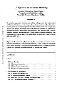
Figure 1. Bivariate bipolar junction transistor (BJT) statistical modeling distributions. Dashed lines are G3s values, symbols are Monte Carlo simulations, and shaded curves are marginal distributions.

performance to fitthat are both key for IC design and that make rsbe, Le, and Jbei observable: the base-emitter voltage Vbes, which gives a defined collector current (this is equivalent to the collector current at a fixed base-emitter bias); the forward Early voltage Vaf (note that this is extracted from measurements, and is not the SPICE model parameter); and b. Table 1 shows measured manufacturing data along with summary statistics from a 10,000-sample Monte Carlo simulation using statistical models, generated from the BPV procedure, based on both linear and quadratic e(p) formulations. The improved accuracy of the quadratic form compared to the linear form for modeling the statistical variations (i.e., the  values) is apparent. Figure 1 shows

39

Authorized licensed use limited to: FREESCALE SEMICONDUCTOR. Downloaded on March 26,2010 at 12:29:37 EDT from IEEE Xplore. Restrictions apply.

mdt2010020036.3d

26/2/010

11:57

Page 40

Compact Variability Modeling for Nanometer CMOS Technology

4.6

Table 2. Extracted standard deviations of L parameters.

4.2

s (mm) 0.017

ODP

0.011

ODN

0.008

4 p

CD

I sats

Parameter

4.4

3.8 3.6 3.4

the shape of the distributions; the skewness in the distributions, which arises from the nonlinearity in the e(p) dependencies (the samples for p are generated from symmetric normal distributions), is clear. To further investigate the capability of the extended BPV procedure, we have modeled PMOS and NMOS devices together, and we included as modeling targets the correlation coefficients between the peak transconductances, gm,max, of wide and long devices and the saturated drain currents, Isats, of wide and short devices. The oxide thickness, tox, was considered common between the PMOS and NMOS device models, and its variance was determined directly from measured capacitance data that is, it was treated as an FPV statistical modeling parameter. Additional parameters (CD, ODP, and ODN) were introduced to model the effective-channel-length variations, and these were transformed into the appropriate SPICE model parameters using the mappings in Equations 1 and 2. Table 2 shows the computed standard deviations of the effective-channel-length parameters’ components. The largest portion of the variation is in the common polysilicon critical-dimension CD variation; however, significant portions of the overall variation are from the out-diffusion parameters, which are separate for each device type. Note that the variations in these individual components of L variation cannot

3.2 3 7.5

8

8.5

9

9.5

10

n Isats

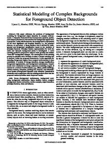
Figure 2. Bivariate scatter plot of PMOS vs. NMOS wide and short saturated drain currents. Symbols are measured data, ellipses are 1s, 2s, and 3s yield curves from 10,000 Monte Carlo samples.

easily be measured directly; they can only be computed using the BPV procedure. Table 3 shows summary statistics for some key types of electrical performance from a 10,000-sample Monte Carlo simulation. The important point is that the correlations are not modeled accurately unless they are explicitly taken into account in the modeling process: The correlations between the peak transconductances are ‘‘naturally’’ fitted because they are for wide and long devices, and we have taken tox to be perfectly correlated between PMOS and NMOS devices. The correlations between the saturated drain currents of the wide and short devices cannot be fitted accurately without the model form in Equations 1 and 2 and the BPV procedure that incorporates fitting of the correlations between e components. The accuracy of the correlation modeling is also visually apparent in the bivariate results of Figure 2, and individual univariate distributions are also modeled well (see Figure 3).

Table 3. MOSFET model statistical results. Device performance

Measured data

Correlated BPV

1.8%

1.8%

NMOS

1.7%

1.7%

PMOS

3.9%

4.1%

NMOS

2.4%

2.4%

p n gm;max Þ rðgm;max;

0.596

0.594

p n Isats Þ rðIsats;

0.718

0.719

Saturated drain currents, Isats 

40

MOSFET type PMOS

Peak transconductances, gm,max 

IEEE Design & Test of Computers

Authorized licensed use limited to: FREESCALE SEMICONDUCTOR. Downloaded on March 26,2010 at 12:29:37 EDT from IEEE Xplore. Restrictions apply.

mdt2010020036.3d

26/2/010

11:57

Page 41

BPV modeling including circuit performance

which has a bordered block-diagonal structure. This structure shows that parameters common to both types of device can also be made observable by including one or more circuit-level performance that depends on the electrical behavior of both types

March/April 2010

1.8 1.6 1.4

PDF

1.2 1 0.8 0.6 0.4 0.2 0

8

8.2

8.4

8.6

8.8

9

9.2

9.4

9.6

9.8

n

I sats

Figure 3. Univariate probability density function for wide and short NMOS saturated drain current. Solid lines are from measured data; dashed lines are from a 10,000-sample Monte Carlo simulation.

5

4

Measurements Normal distribution fit for measurements Normal distribution fit for Monte Carlo simulation W/L=10/0.2 µm

Density

The theoretical formalism we have presented makes no assumptions about what are selected as the components of e. Conventionally, these are device-level measurements (embodying either global or local variation). Typically, these device performances are chosen so that they make the process parameters, p, observable and serve as key quantities that control circuit performance. Nothing, however, technically prevents some or all components of e from being measures of circuit performance. Indeed, incorporating circuit-level performance as part of the statistical-modeling process can only improve the overall accuracy of modeling circuit behavior. Accurate modeling of circuit performance is the ultimate goal of modeling, not modeling device-level performance or parameter variations. To that end, we have used the PSP MOSFET model to characterize the statistical variation of PMOS devices, NMOS devices, and ring oscillators, which are all measured from the same sample wafers. PSP is the most accurate and physical MOSFET model available,10 and so should be expected to provide good statistical-modeling capability while using as few parameters as possible. Conceptually, the process parameters can be broken into three groups: those that affect only PMOS devices, pp; those that affect only NMOS devices, pn; and those that are common and affect both types of devices, pc. Similarly, the different components of electrical performance can be broken into three categories: those specific to PMOS devices, ep; those specific to NMOS devices, en; and those that are circuit performances, ec, which depend on the performance of both the PMOS and NMOS transistors. The propagation of variance relations in Equation 6, considering only linear variations, becomes 2 3 !2  2 @e @e p p 6 7 0 @pp @pc 7 2 3 6 3 6 72 6  2  2 7 s2pp s2ep @en @en 7 6 2 7 6 2 7 76 4 sen 5 ¼ 6 6 0 74 spn 5 @p @p n c 6 7 2 s2ec ! 6 7 s (17) 6 @e 2  @e 2 @e 2 7 pc c c c 4 5 @pp @pn @pc

2

3

2

1

0 4.5

4.75

5 Isats (mA)

5.25

5.5

Figure 4. Measured and modeled distributions for wide and short NMOS saturated drain current.

of device, in contrast to explicitly including correlations between e components, as was done in the ‘‘Extended BPV results’’ section. The coupled device-circuit-level statistical BPV modeling procedure was applied to our measured data from individual devices and ring oscillators. Figure 4 shows the measured and modeled results

41

Authorized licensed use limited to: FREESCALE SEMICONDUCTOR. Downloaded on March 26,2010 at 12:29:37 EDT from IEEE Xplore. Restrictions apply.

mdt2010020036.3d

26/2/010

11:57

Page 42

Compact Variability Modeling for Nanometer CMOS Technology

Measurements Simulations with additional drain currents for multiple VGS being fitted Simulations with a single drain current being fitted

14

s td (ps)

at the highest VDD value. We stress that we added only extra drain currents as modeling targets; we didn’t explicitly include variances in the gate delays td at the lower supply voltages as additional fitting targets, but they follow from the improved fitting of NMOS and PMOS Isats over VDD.

10

6

2 1

1.2

1.4

1.6

1.8

VDD (V)

THE BPV FORMALISM was previously verified to work well for both global and local (mismatch) statistical modeling, and has now been verified to be able to handle nonlinearities and correlations, and to be able to be applied using circuit-level as well as device-level measures of electrical performance. Remaining challenges include extension to handle both global and local variations in a single and unified manner, and to be able to leverage the analysis of nonlinearities and correlations to predict optimum corner models taking both of these effects into account. 

Figure 5. Measured and modeled ring oscillator gate delay variation as a function of supply voltage.

 References 1. W. Maly and A.J. Strojwas, ‘‘Statistical Simulation of the

for the saturated drain current of wide and short NMOS devices. The accuracy of the statistical model is clear. Figure 5 shows the measured and modeled variation in the ring oscillator gate delay, td, as a function of the supply voltage VDD. The dashed line shows the model results when the PMOS and NMOS saturated drain currents and the ring oscillator gate delay are fitted only at the highest value of VDD. The BPV procedure obviously fits the statistical variation of td well, at the highest supply voltage; however, the accuracy degrades for lower supply voltages. Even though PSP is an extremely accurate model, and it fitted the measured device’s current-voltage and capacitancevoltage characteristics well, and also perfectly fitted the variances of Isats and td at a high VDD, clearly there is imprecision in extrapolating the variances to lower VDD values. Besides there being no restriction on what the components of e are, the BPV technique has no restriction on how many components of e can be included in the modeling procedure (as long as it is at least the minimum number to make all the process parameters, p, observable). The solid line in Figure 5 shows the statistical variation in the gate delay when additional drain currents, at lower supply voltages, are added to the BPV procedure. Clearly, fitting the variance of td over VDD shows significant improvement, with essentially no loss in modeling accuracy

42

IC Manufacturing Process,’’ IEEE Trans. Computer-Aided Design, vol. 1, no. 3, 1982, pp. 120-131. 2. C.K. Chow, ‘‘Projection of Circuit Performance Distributions by Multivariate Statistics,’’ IEEE Trans. Semiconductor Manufacturing, vol. 2, no. 2, 1989, pp. 60-65. 3. M. Bolt, M. Rocchi, and J. Engel, ‘‘Realistic Statistical Worst-Case Simulations of VLSI Circuits,’’ IEEE Trans. Semiconductor Manufacturing, vol. 4, no. 3, 1991, pp. 193-198. 4. C.C. McAndrew et al., ‘‘Efficient Statistical BJT Modeling, Why b Is More That Ic/Ib,’’ Proc. IEEE Bipolar/BiCMOS Circuits and Technology Meeting, IEEE Press, 1997, pp. 28-31. 5. C.C. McAndrew, ‘‘Efficient Statistical Modeling for Circuit Simulation,’’ Design of Systems on a Chip: Devices and Components, R. Reis and J. Jess, eds., Kluwer Academic, 2004, pp. 97-122. 6. C.C. McAndrew and P.G. Drennan, ‘‘Device Correlation: Modeling Using Uncorrelated Parameters, Characterization Using Ratios and Differences,’’ Proc. Workshop Compact Modeling (Nanotech 06), Nano Science and Technology Institute, 2006, pp. 698-702. 7. W.F. Davis and R.T. Ida, ‘‘Statistical IC Simulation Based on Independent Wafer Extracted Process Parameters and Experimental Designs,’’ Proc. IEEE Bipolar/BiCMOS Circuits and Technology Meeting, IEEE Press, 1989, pp. 18-19. 8. I. Stevanovic and C.C. McAndrew, ‘‘Quadratic Backward Propagation of Variance (QBPV) for Nonlinear Statistical

IEEE Design & Test of Computers

Authorized licensed use limited to: FREESCALE SEMICONDUCTOR. Downloaded on March 26,2010 at 12:29:37 EDT from IEEE Xplore. Restrictions apply.

mdt2010020036.3d

26/2/010

11:57

Page 43

Circuit Modeling,’’ IEEE Trans. Computer-Aided Design, vol. 28, no. 9, 2009, pp. 1428-1432. 9. X. Li et al., ‘‘Statistical Modeling with the PSP MOSFET Model,’’ IEEE Trans. Computer-Aided Design, vol. 29, 2010, to appear. 10. G. Gildenblat et al., ‘‘PSP: An Advanced SurfacePotential-Based MOSFET Model for Circuit Simulation,’’

Ivica Stevanovic´ is a scientist at the ABB Corporate Research Center in Da¨ttwil, Switzerland, and an external research member with Ecole Polytechnique Fe´de´rale de Lausanne (EPFL). His research interests include numerical and statistical modeling. He has a PhD in electrical engineering from EPFL. He is a member of the IEEE.

IEEE Trans. Electron Devices, vol. 53, no. 9, 2006, pp. 1979-1993.

Colin C. McAndrew is a Distinguished Member of Technical Staff at Freescale Semiconductor. His research interests include semiconductor device modeling and statistical modeling for circuit simulation. He has a PhD in systems design engineering from the University of Waterloo, Ontario. He is a Fellow of the IEEE.

Gennady Gildenblat is the Motorola Professor of Electrical Engineering at Arizona State University. His research interests include semiconductor device physics and modeling, novel semiconductor devices, and semiconductor transport. He has a PhD in solid-state physics from Rensselaer Polytechnic Institute. He is a Fellow of the IEEE.

Direct questions and comments about this article to Xin Li is a SPICE modeling engineer at GlobalFoundries and is pursuing a PhD in electrical engineering at Arizona State University. His research interests include MOSFET compact modeling and statistical modeling. He has an MS in electrical engineering from Pennsylvania State University.

March/April 2010

Colin C. McAndrew, Freescale Semiconductor, 2100 East Elliot Rd., Tempe, AZ 85284; colin.mcandrew@ freescale.com.

43

Authorized licensed use limited to: FREESCALE SEMICONDUCTOR. Downloaded on March 26,2010 at 12:29:37 EDT from IEEE Xplore. Restrictions apply.