Jan 6, 1991 - method uses a factorial method to search the design space, with a confined definition of an .... Fractional factorial designs [1] are used to reduce.
Extensions to the Taguchi Method of Product Design∗ Kevin N. Otto† Erik. K. Antonsson ‡ Engineering Design Research Laboratory Division of Engineering and Applied Science California Institute of Technology January 6, 1991
Abstract The Taguchi method of product design is an experimental approximation to minimizing the expected value of target variance for certain classes of problems. Taguchi’s method is extended to designs which involve variables each of which has a range of values all of which must be satisfied (necessity), and designs which involve variables each of which has a range of values any of which might be used (possibility). Tuning parameters, as a part of the design process, are also demonstrated within Taguchi’s method. The method is also extended to solve design problems with constraints, invoking the methods of constrained optimization. Finally, the Taguchi method uses a factorial method to search the design space, with a confined definition of an optimal solution. This is compared with other methods of searching the design space and their definitions of an optimal solution.
∗
EDRL-TR 90f: Manuscript to appear in the ASME Journal of Mechanical Design. Graduate Research Assistant ‡ Associate Professor of Mechanical Engineering, Mail Code 104-44, Caltech, Pasadena, CA 91125 †
1
Otto & Antonsson: Extensions to the Taguchi Method of Product Design
Nomenclature DP PP ~x,~xj p~,~ pi ~n,~nk ~t,~tk S/N ratio m n l pri ,dP r τ ~x∗
Design parameter. A parameter whose value is chosen during the design process. Performance parameter. A parameter whose values depend on the design parameter values, and give indications of performance. Vector of design parameters. ~xj refers to a particular arrangement chosen to use at experimental arrangement j. Vector of noise parameters. p~i refers to a particular arrangement chosen to use at experimental arrangement i. Vector of necessary parameters. ~nj refers to a particular arrangement chosen to use at experimental arrangement k. Vector of tuning parameters. ~tj refers to a particular arrangement chosen to use at experimental arrangement k. Signal to noise ratio. Dimension of the noise parameter vector p~. Dimension of the design parameter vector ~x. Dimension of the necessary ~n or tuning ~t parameter vector. Probability of experiencing experimental arrangement p~i (discretized case) or p~ respectively. Target value for the performance parameter P P .
q T
Solution design parameter vector. The objective function performance parameter when discussing constrained problems. The constraint performance parameters when discussing constrained problems. Number of constraint equations. The boundary method unconstrained optimization function.
P K
The boundary method penalty function. The boundary method penalty function scaling factor.
ne
The number of violated constraints in ~g. The number of experiments (out of m possible) which do not satisfy the constraints ~g. Prescribed acceptable probability of failure.
f ~g
emax D
2
Otto & Antonsson: Extensions to the Taguchi Method of Product Design
3
1 Introduction Taguchi’s method has become increasing popular as a method for developing engineered products. It promises, and delivers, an ability to increase the quality of an engineered product via simple changes in the method by which engineers perform their usual design tasks. Given the bold claims, there has been relatively little research in the design community on Taguchi’s method: its foundations, assumptions, mathematics, techniques, and approximations. There has been little research to compare the technique to other methods, either analytically or experimentally, except for comparisons with experimental design techniques from which Taguchi’s method is derived. In addition, there has been little research to attempt to improve the method itself. This paper will address these issues. It will discuss Taguchi’s method by comparing it analytically with such methods as optimization, experimental design, and the method of imprecision [22]. Taguchi’s method will be extended to permit it to address problems, such as designs with constraints, that these other methods can handle but which Taguchi’s method currently cannot. The searching techniques used by the various methods will also be discussed. Before such a discussion can occur, other methods must be placed in perspective. Optimization, for example, searches for an optimal set of design parameters (DP s) by finding the minimal value of a performance parameter (P P ), the merit function [4, 10]. The feature which makes optimization most powerful in comparison to other methods is its ability to handle multiple performance parameters in the form of constraints. Taguchi’s method and basic experimental design have no such mechanism. If there are confounding influences (probabilistic noise) in the design, optimization methods can model these noise parameters (N P s) as well [13]. Experimental design [1, 5, 7] is another method available to determine which set of design parameters to use. Here one experiments with different sets of design parameter values, and chooses the set which maximizes an objective, even with confounding influences (probabilistic noise). However, none of the above methods address concepts of necessity and possibility, first introduced to the design community by A. Ward and K. Wood along with one of the authors [19, 20, 22, 24]. For example, consider a motor design which must meet every value within a range of different speed and torque combinations. A necessity requirement, such as this, is not handled by the above methods. Just as necessity is a method to represent requirements in a design, possibility is a method to represent arbitrary freedoms to which a design will be subject. For example, consider operator adjustment variables such as seat positioning within an automobile. Possibilistic parameters are different from design parameters in that a design parameter must, at the end of the design stage, be chosen to have a value. A possibilistic parameter, however, is never chosen, it is always free to change. Further, they change to increase performance. The seat position chosen by an operator is not a parameter the design engineer chooses, yet its positioning can increase performance. A possibilistic freedom, such as this, is not handled by the above methods. The method of imprecision [22, 23, 24, 25] is a technique for selecting values of the design parameters based on zero to one rankings of the values of the design and performance parameters, rather than on the values of the parameters themselves. This allows other information to also be included, such as necessity, possibility, and probability. Taguchi’s method will now also be reviewed, and subsequently extended to show its relation among other various methods. Below we briefly review the philosophy and mathematics of Taguchi’s method to show its relation to the other methods described above. We will then extend Taguchi’s method to incorporate constraints, and some aspects of necessity and possibility.
Otto & Antonsson: Extensions to the Taguchi Method of Product Design
4
2 Review of Taguchi’s Method Taguchi’s method makes use of an experimental process for finding an optimal design. The reader is referred to [2, 6, 11, 17] for a complete discussion, as this section is only presented to review the methodology and nomenclature. The search objective is to maximize a design metric over the design space, where each evaluation in the design space incorporates the noise space variations. Hence, for each experimental point in the design space (called “inner array” by Taguchi), the design metric (called the “S/N ratio” by Taguchi), as a function of the experimental arrangement of the DP s ~xj , is S/N (~xj ) ≡ −10 log
"m X
#
2
(P P (~xj , p~i ) − τ ) × 1/m
(1)
i=1
where P P is the one performance parameter being considered, m is the number of noise parameter arrangements p~i , and τ is the desired target value [2]. The points in the noise space p~i (called “outer array” by Taguchi) are chosen using a factorial method (called “orthogonal arrays” by Taguchi). Fractional factorial designs [1] are used to reduce computation. Taguchi provides justification for using his design metric based on the first two terms of a Taylor series expansion of societal loss (see [17]). It is assumed in this derivation that the preliminary design has been completed, and the optimal values of the design parameters need to be determined. Note that the basic experimental methodology can be used even in preliminary design, but it would not lead to designs which minimize total societal loss. This will be discussed further below. The search over the design space is intended to maximize the metric of Equation (1) above. The issue of how to search across the design space is an entirely separate issue from how to model the noise space variations. In Taguchi’s method, the search across the design space is performed in precisely the same fashion as the approximation of the noise space is performed: using a factorial method. That is, the arrangement of design parameters with the highest S/N ratio is chosen. Of course, another round of experiments can be performed around that optimal point for a finer resolution, provided that certain conditions are met, as will be discussed below.
2.1 Analysis of Uncertainty Incorporated in Taguchi’s Method Recall the basic Taguchi definition of an S/N ratio at each DP arrangement, Equation (1). This defines a surface over the design space by evaluating the function P P at each experimental arrangement of the DP s (~xj ), which is evaluated by summing over the noise: at each p~i . The set ~xj which maximized the S/N ratio (the sum over p~) is chosen. This definition itself, however, is an approximation of the weightings assigned to each particular experimental arrangement of noise, based on the probability of experiencing that experimental arrangement. This basic Taguchi approach assigns a weighting of 1/m to each experimental arrangement, regardless of the likelihood of any particular experimental arrangement. Instead of the basic Taguchi method as reflected by Equation (1), Taguchi’s method can be extended to be more accurate by using the probability of each experimental arrangement occurring. That is, use an S/N ratio of: "
S/N (~xj ) ≡ −10 log
m X i=1
#
2
(P P (~xj , p~i ) − τ ) × pri
(2)
Otto & Antonsson: Extensions to the Taguchi Method of Product Design
5
where pr i is the probability of experiencing noise factor arrangement i (replacing 1/m in the basic Taguchi method). This is determined by probabilistically combining the probability density functions of the individual noise factors. Note that the probability density functions must be discretized into a probability, based on how much of the probability density function’s area under the curve the experimental point is intended to represent. This provides the key to determining what experimental noise parameter values should be used. To determine where the experimental points should be, the density function should first be split into areas, and then the expected values of each of the areas should be found. These expected values should then be used as the experimental points, and each assigned a weighting equal to the area they represent. See Figure (1). Note that these decisions on how to split up the areas are imprecise. Since in the basic Taguchi method each noise factor must be independent of one another, combining these probability assignments into the pri (for each noise parameter arrangement p~i ) requires simple multiplication. For best results, the density functions should be split into equal areas, and then all experimental points will, of course, have the same weighting. Unfortunately, this is not always possible, since the density functions may not be known until the experiments are completed (and perhaps not even then). Equation (2) is therefore seen as a way to make Taguchi’s method more accurate in uncertain experimental environments. The experiments are first performed, and subsequently are weighted based on this experimental experience. Usually the probability density functions are assumed to be normal, and the experimental points are assumed to be chosen at a nominal value and plus and minus a deviation such that all have the same probability of occurring (1/3), and pr i is the same 1/m for all of the experiments (for a 3 factorial design). This may not be true in general, if, for example, the experimenter decides to also consider cases which are not very likely, either by choice or by lack of knowledge about the noise space. These observations lead to an exact definition of what needs to be evaluated across the noise space of the design. Provided that the noise consists entirely of probabilistic uncertainty, Taguchi’s method is an experimental approximation to an exact expression of: S/N (~x) ≡ −10 log
"Z
# 2
P r(~ p|~ x)
(P P (~x, p~) − τ ) dP r(~ p|~x)
(3)
This observation was also made by N. Singpurwalla in an earlier paper [14]. Thus Taguchi’s method is an experimental approximation which is intended to select the DP arrangement defined implicitly by:1 ∗
S/N (~x ) ≡ max
~ x∈DP S
−10 log
"Z
#! 2
P r(~ p|~ x)
(P P (~x, p~) − τ ) dP r(~ p|~x)
(4)
where P r(~ p|~x) denotes the probability of experiencing noise parameter arrangement p~, given the value of the design parameters ~x. This formulation accommodates cases for which P r(~ p) changes with positions in the design space. For example, manufacturing noise may increase with a design parameter change of material. Note that Equation (3) is expressing the expected value of (P P (~x, p~) − τ )2 over the noise space (through a transformation: −10 log). Hence Taguchi’s method is an experimental approximation 1
Note that throughout the paper max is used to to mean sup or least upper bound, and min is used to mean inf or greatest lower bound.
Otto & Antonsson: Extensions to the Taguchi Method of Product Design
6
to finding the point ~x∗ which minimizes the expected value of the target variance over the design’s probabilistic noise. Having established what Taguchi’s method is intended to approximate, extending the method to more complex design problems is possible. For example, possibilistic uncertainties or intervals of necessity have not been examined. Also, there has been no discussion of the validity of the search technique across the design space (e.g., how to evaluate the maximization in Equation (4)). The next sections will discuss these points.
3 Different Uncertainty Forms As discussed in the introduction, there are different kinds of uncertainties: imprecision, probabilistic, necessary, and possibilistic uncertainties. As already shown, Taguchi’s method models probabilistic uncertainty. The following section will investigate whether these other forms of uncertainty can be incorporated into Taguchi’s method.
3.1 Imprecision and Taguchi’s Method Imprecision is a methodology which allows designers to quantitatively incorporate their engineering judgment (preference) during the design process [22, 23, 24, 25]. The Taguchi method, however, is a methodology which allows judgments based on total societal loss – society’s preference. Therefore, to maintain the societal loss concept of Taguchi’s method, imprecision cannot be incorporated. Taguchi’s method maintains that the designer will prefer only the solution which minimizes variance, since this approximates minimizing cost to society as a whole, even if it costs the designer or manufacturer more, and hence reduces the designer’s preference. Imprecision, however, is used to represent the designer’s preference, due to such reasons as manufacturing cost. There is a fundamental difference between the philosophy of Taguchi’s method and the philosophy of imprecision. In Taguchi’s method, societal loss inherently is the only consideration which affects the choice of design parameter values (variations in the product due to noise are minimized, regardless of other concerns), design or manufacturing considerations are excluded. Therefore, the two methods are incompatible. Either designers will make choices based on their judgment and preferences, or they will make choices based on an approximation of society’s preference.
3.2 Necessity Intervals and Taguchi’s Method Suppose there is a subset of parameters in the design which have an interval of values which all must be satisfied. For example, suppose in an electric motor design, a range of speed and load requirements must all be met [20]. The performance derivable from a design should be ranked as the worst case out of all which must be satisfied. This observation allows Taguchi’s method to be extended to designs which have such necessity requirements. That is, we extend Taguchi’s method to such problems by defining an S/N ratio of: "
S/N (~x) ≡ −10 log max ~ n|~ x
"Z P r(~ p|~ x,~ n)
## 2
(P P (~x, p~, ~n) − τ ) dP r(~ p|~x, ~n)
(5)
Otto & Antonsson: Extensions to the Taguchi Method of Product Design
7
Here ~n is an arrangement of the necessary parameters, chosen out of the space spanned by the (possibly co-dependent) intervals of necessity of each necessary parameter. The intervals can, of course, vary with ~x, and thus the ~n|~x formulation. The DP set to use is defined implicitly by: " ∗
S/N (~x ) ≡ max
~ x∈DP S
"
−10 log max ~ n|~ x
"Z
### 2
P r(~ p|~ x,~ n)
(P P (~x, p~, ~n) − τ ) dP r(~ p|~x, ~n)
(6)
Note that the basic Taguchi method does not include a method for incorporating these kinds of requirements. They can, however, be approximated in the same fashion as Taguchi’s method, by incorporating the methods of experimental design: "
"
S/N (~x) ' −10 log max
k=1,l
m X i=1
##
(P Pik (~x) − τ )2 × pri
(7)
where k indexes across the necessary experimental arrangements, and i indexes across the probabilistic noise experimental arrangements. The DP set to use is given by: " ∗
S/N (~x ) ' max
~ x∈DP S
"
−10 log max
k=1,l
"
m X i=1
### 2
(P Pik (~x) − τ ) × pri
(8)
The difference between probability and necessity is also easily observed in the experimental approximation: probabilistic uncertainty experiments are weighted based on their probability. The experiments in necessity are ignored except for the worst case experiment, (which is unknown and therefore must be found by experimenting). Note also that this is the proper mechanism to model probabilistic variables that must be satisfied over a range of their distributions. For example, a parameter np might be the vertical accelerations an automobile tire subjects to an axle. The axle must be designed to all possible values of the acceleration to prevent failure, but note that such accelerations are usually modeled in a probabilistic fashion. The accelerations np vary probabilistically and must, for example, be satisfied to within 3 standard deviations, and so np must be modeled as a necessary variable, not as a probabilistic variable as in the basic Taguchi method. The interval(s) of necessity of np would be all np such that pdf (np ) ≥ 0.05, for a 3 standard deviation design.
3.3 Possibilistic Uncertainty and Taguchi’s Method Suppose that there is a subset of parameters in the design which has an interval in which the value is always free to vary. For example, in an electric motor design, any current between zero and 15 amps could be drawn (since, in this example, a circuit protector would trip above 15 amps). In such types of uncertainties the design is free to adopt any value within the range of possibility. The difference between a design parameter (one that the designer chooses) and a parameter which can vary possibilistically (one which is free to adopt any value within the range of possibility) is very subtle. Possibilistic uncertainties are never fixed, they always opportunistically vary over their ranges. This has implications when the precedence order of the variables is considered, as will be discussed next. If a possibilistic uncertainty occurs before the probabilistic uncertainty has occurred, Taguchi’s method has no mechanism to distinguish between a possibilistic uncertainty and a design parameter.
Otto & Antonsson: Extensions to the Taguchi Method of Product Design
8
Both are represented by intervals, and the value which maximizes the S/N ratio is used, and it will not vary as p~ varies. In the electric motor example, the mass cannot change to overcome probabilistic variations which occurred in the motor’s manufacture, as compared to the desired specifications of the motor, even though the mass has a range of possibility. Mass is a design parameter. If, on the other hand, the possibilistic uncertainty occurs after the probabilistic uncertainty has occurred, Taguchi’s method can be extended to distinguish between possibilistic uncertainties and design parameters. The possibilistic uncertainty parameters are then tuning parameters. Modeling of tuning parameters in various formulations (such as optimization, the method of imprecision, and Taguchi’s method) is introduced in [9]. When the possibilistic uncertainty represents a tuning parameter, the probabilistic uncertainty occurs first and subsequently the possibilistic uncertainty parameter can adjust to overcome the probabilistic parameter’s confounding influence. In the electric motor example, the current drawn by the motor can vary to provide a specified speed despite fluctuations in applied load. The best examples of a possibilistic uncertainty as a tuning parameter are post-manufacturing adjustment variables, such as set screws on automobile carburetors. Their setting is not specified by the designer, but is set after the engine is manufactured to maximize performance and/or economy. The setting is a tuning parameter, and it has a range of possibility. The key aspect of a tuning parameter is that when a probabilistic parameter p~ varies, a possibilistic tuning parameter ~t can also vary to overcome p~’s confounding influences. This observation allows Taguchi’s method to be extended to such variables. That is, we extend Taguchi’s method to such problems by defining an S/N ratio of: S/N (~x) ≡ −10 log
"Z
h
#
i
min (P P (~x, p~, ~t) − τ )2 dP r(~ p|~x)
(9)
P r(~ p|~ x) ~t|~ x,~ p
Note that ~t is not fixed at a value and then p~ confounds the result (which is what occurs with design parameters). Rather ~t can vary to overcome ~p’s confounding influences to bring the result exactly on target. The DP set to use is implicitly defined by: " ∗
S/N (~x ) ≡ max
~ x∈DP S
−10 log
"Z
h
##
i
min (P P (~x, p~, ~t) − τ )2 dP r(~ p|~x)
P r(~ p|~ x) ~t|~ x,~ p
(10)
Note that the basic Taguchi method does not include a method for incorporating possibilistic uncertainties. These can, however, be approximated in the same fashion as Taguchi’s method does by incorporating the methods of experimental design: "
S/N (~x) ' −10 log
m X i=1
h
#
i
min (P Pik (~x) − τ )2 × pr i
(11)
k=1,l
where k indexes across the possibility experiments, and i indexes across the probabilistic noise experiments. The DP set to use is given by: " ∗
S/N (~x ) ' max
~ x∈DP S
−10 log
"
m X i=1
h
2
min (P Pik (~x) − τ )
k=1,l
i
##
× pri
(12)
This is a mathematical modeling of the concept of tuning parameters in engineering design using Taguchi’s method. In fact modeling these parameters in Taguchi’s method is counter to the Taguchi
Otto & Antonsson: Extensions to the Taguchi Method of Product Design
9
philosophy. Ideally tuning parameters should be eliminated (by proper selection of the nominal values of the design parameters) since use of tuning parameters adds to the manufacturing cost. However, if it is known that a tuning parameter will be necessary, the rest of the design parameters should be chosen based on this knowledge. Expensive design parameters can be avoided, in some circumstances, if the design is going to have to be tuned. The above formulation incorporates this consideration; experimental parameter design, as presented by Taguchi, does not.
3.4 Hybrid Forms of Uncertainty If the design problem encountered has multiple variable forms (probabilistic, possibilistic, and necessary), then Equations (7) through (11) can be combined. To do so, however, requires the precedence relation among the variables to be established. The order among the probabilistic, possibilistic, and necessary parameters must be established. The precedence relation is the order in which the variability of the parameters occurs: the temporal order in which the parameter values are established. For example, in the electric motor example, the values ~x of the motor geometry are first selected, followed by the probabilistic manufacturing errors p~ occurring. Suppose also there is a necessary parameter ~n representing a range of speed and loading. After manufacture, the loading is applied, to which the current drawn ~t responds, to maintain a target speed. The precedence relation is then ~x, ~n, p~, ~t. The optimal set of design parameters ~x∗ to use would be given by, using the extended Taguchi approach: "
S/N (~x∗ ) = max −10 log max ~ x
~ n|~ x
"Z
h
i
#!#
min f (~t, p~, ~n, ~x) dP r(~ p|~n, ~x)
P r(~ p|~ n,~ x) ~t|~ p,~ n,~ x
(13)
It is not always the case, however, that this will be the precedence relation among the variables. Individual necessity variables may also vary in their precedence relative to individual possibilistic and probabilistic variables, and possibilistic variables among the probabilistic. The order is problem dependent. This requirement that the precedence relation be established among the variables is a general problem of designs with multiple uncertainty forms, and must be considered no matter what the formalism. It exists with optimization, Taguchi’s method, and the method of imprecision when they incorporate these multiple uncertainty forms.
4 Incorporating Other Search Techniques The standard Taguchi method spans the entire design space and noise space by experiments. After performing a series of experiments, the best arrangement of DP s are chosen. Interpolation between experiments is possible, with an extra experiment or set of experiments performed at, or around, the interpolated point. This methodology can be replaced by different search techniques. What must be evaluated is the maximization of Equation (4). Consider Taguchi’s method using a full 2 factorial design method on the design space (and as many as required on the noise space). Taguchi’s method can then be interpreted as the first step of a binary search algorithm.2 It selects one of the two DP values along each axis of the design space. Hence a more effective approach would be to continue this process 2
This observation was first brought to the attention of the authors by personal communication with Prof. K. L. Wood, University of Texas at Austin.
Otto & Antonsson: Extensions to the Taguchi Method of Product Design
10
using binary search. Or one could use a hill climbing strategy on the design space, rather than factorially considering all alternatives, some of which will be poor. Hill climbing focuses the search to the better regions of the design space. Techniques of globally optimal hill-climbing can also be used to find the guaranteed globally optimal solution [3, 26]. Hill climbing with Taguchi’s method is discussed in [18], where a probabilistic perturbation using Taguchi’s method is considered at each step of a hill-climbing search. However, the authors of [18] modeled design parameters without noise in the same way as design parameters with noise. Design parameters will not have noise if any probabilistic variations of the design parameter are negligible; for example, with a design parameter manufactured with a very accurate machine, relative to the other manufacturing equipment. The required number of experiments falls drastically when this observation is made: one need not perturb each evaluation point of such design parameters. Once the realization of the separation of the noise parameters (~ p, ~n, and ~t) from the design parameters (~x) is made, this possible savings in experiments is immediately clear. The standard adoption of Taguchi’s method, however, does not perform a full factorial analysis. Necessary and sufficient conditions required of the performance parameter such that the partial factorial analysis produces the optimal solution are not known.
4.1 Designs with Constraints The problem with the extended Taguchi methodology that uses hill climbing, however, is the same problem which exists with the basic Taguchi method: choosing the experimental points in the design space. The method assumes that an unconstrained search is possible, which may not be the case if there are constraint variables which limit the choice of the DP s. Simply declaring the use of orthogonality (which means use a factorial method) or basic hill climbing to determine the experimentation points is not a sufficient answer, since these methods may choose points which violate a constraint. Methods of constrained search must be invoked to choose the new set of experimental points. Note that constraints on the DP s exist in the basic Taguchi method, they just are not explicitly identified. It is assumed the DP ranges were chosen so that all of the experimental points are feasible. Therefore the only constraints expressed in Taguchi’s method and experimental design in general are direct inequality constraints on the DP s (such as xi ≤ 0). Constraint expressions like g(~x) ≤ 0 are not incorporated (note the evaluation of g may require an experimental process if no analytic expression is available). Of course, one can evaluate g(~x) at each experimental point to ensure it is feasible. The addition of uncertainty in the constraint expression, however, makes this difficult (g(~x, p~) ≤ 0). The basic Taguchi method (and even experimental design in general) is intended for one P P only, the merit function; not additional constraint P P expressions. Incorporation of these constraints is an extension of the Taguchi method. By reformulating the Taguchi method to include constraint expressions, we can extend Taguchi’s method to include multiple constraints. Let f (~x, p~) be a merit function of interest. Additionally, there are constraints of the form ~g (~x, p~) ≤ ~0. Equality constraints are not discussed, but are easily incorporated. Necessary and possible variables are also easily included using one of the S/N ratios of Equation (5) through Equation (9) instead of the S/N ratio only for probabilistic noise (Equation(2)) used in this derivation. Also, the evaluations of ~g (~x, p~) can be experimental in nature. Then the well established methods of constrained search can be used to guide the search to an optimum [12].
Otto & Antonsson: Extensions to the Taguchi Method of Product Design
11
To define the constrained optimization problem, maximize S/N (~x) ≡ −10 log
"Z
# 2
P r(~ p|~ x)
(f (~x, p~) − τ ) dP r(~ p|~x)
(14)
subject to min[P r(~gj (~x, p~) ≤ 0)] ≥ D
(15)
j
where D is a specification of an acceptable probability of meeting the constraints ~g, and j indexes across the constraint equations. Others have worked on extending Taguchi’s method to include constraints. Wilde [21] formalizes Taguchi’s method into minimizing the largest possible absolute deviation from target, and then develops analytic solutions for the case of monotonic parameters. That analysis is based on minimizing the maximum deviation. Our analysis of Taguchi’s method (presented here) is based on the sum used by Taguchi (Equation (1)). Having defined the problem, it can be solved, for example, by the use of a boundary method of constrained optimization. Boundary methods [10] will work, and should suffice, even with their difficulty in convergence near the optimum. This method will find the optimum region within a few iterations, which is usually all that is required for problems using experimental techniques such as Taguchi’s method. To define an appropriate boundary method, let "
T (~x) = −10 log
i=1
(
where P (~x) =
#
m X
−K × ne × ln 0
2
(f (~x, p~i ) − τ ) × pri + P (~x) � m−emax � mD
if emax ≥ m(1 − D) if emax ≤ m(1 − D)
(16)
(17)
where emax is the number of experiments which do not satisfy a constraint ~gj and where ~gj is the constraint which failed the most number of times out of the q constraint equations in ~g (so 0 ≤ emax ≤ m). K is a large number relative to −10 log[f ], and ne is the number of constraints in ~g which are not met (these simply help speed convergence). Maximizing T will converge to the optimal point, i.e., the set of DP s ~x which minimize variations due to noise p~, but subject to the probabilistic constraints ~g (~x, p~) ≤ ~0. Practically, such a boundary formulation is difficult to solve when there are a small number of experiments (m) used to approximate the noise p~. P ranges from zero to infinity in m steps, and if m is small, searching techniques usually have difficulty approaching a constraint boundary. Note that the entire problem can also be formulated using a Monte-Carlo technique. In fact, if the merit function is not the S/N ratio (the expected value of the variance of the P P ), but is instead the expected value of the P P , then the method is exactly the method of probabilistic optimization, as presented in [12], chapter 13. For minimization problems, the two methods are identical if Monte-Carlo simulation is used. Taguchi would minimize P P (~x, p~)2 , and probabilistic optimization minimizes P P (~x, p~). Minimizing one minimizes the other. Hence there is no difference between probabilistic optimization (as presented in [12]) and Taguchi’s method with constraints, hill climbing, and Monte-Carlo simulations of noise.
Otto & Antonsson: Extensions to the Taguchi Method of Product Design
12
5 Design Example This example considers the design of a pressurized air tank, and is the same problem as presented in Papalambros and Wilde [10], page 217. The reader is referred to the reference to see the restrictions applied to this problem to permit it to be solved using crisp constraints and an optimization methodology. The example is very simple but was chosen for this reason and the ability of its merit function and constraints to be represented on a plane for an easy graphical explanation. The design problem is to determine which of two designs to pursue – an air tank design with hemispherical heads, or an air tank design with flat heads. See Figure (2). There are four performance parameters in the design. The first is the metal volume m: m = 2πKs r 2 l + 2πCh Kh r 3 + πKs2 r 2 l
(18)
This parameter is proportional to the cost and is to be minimized. Another parameter is the capacity (volume) of the tank v: v = πr 2 l + πKv r 3 (19) This parameter is a measure of the attainable performance objective of the tank, to hold air, and is modeled as a constraint with an aspiration level. Another parameter is an overall height restriction L0 : l + 2(Kl + Kh )r ≤ L0 (20) Finally, there is an overall radius restriction R0 : (Ks + 1)r ≤ R0
(21)
The last two performance parameters have their limits set by spatial constraints. The coefficients K are from the ASME code for unfired pressure vessels. S is the maximal allowed stress, P is the applied pressure, and E is the joint efficiency. (
Kh = (
Kl =
p
2 CP/S P 2S−.2P
0 flat 4/3 hemi
P 2SE − .6P ( 0 flat = 1 hemi
flat hemi
(22) (23)
Ks =
(24)
Kv
(25)
Hence the design space of this example is spanned by 2 design parameters l and r. The problem, however, is confounded by noises. That is, there are manufacturing errors on l and r which limit how well one can specify their values. This error is taken to be Gaussian, although any distribution that matches the data could be used. There is also error introduced by the variability of the material supplied. This error is manifested in the allowable stress S, which is taken to vary as a beta distribution. Finally, there is error introduced in the variability of the welds made. This error is manifested in the joint efficiency E, which also is taken to vary as a beta distribution. These distributions are shown in Figures (3) through (5).
Otto & Antonsson: Extensions to the Taguchi Method of Product Design
1
2
13
3
Figure 1: Determining noise parameter experimentation values.
r l
Figure 2: Flat and Hemispherical head air tank designs.
r l
Otto & Antonsson: Extensions to the Taguchi Method of Product Design
Figure 3: Length l and radius r uncertainty distribution.
14
Otto & Antonsson: Extensions to the Taguchi Method of Product Design
Figure 4: Allowable stress S uncertainty distribution.
15
Otto & Antonsson: Extensions to the Taguchi Method of Product Design
Figure 5: Joint efficiency E uncertainty distribution.
16
Otto & Antonsson: Extensions to the Taguchi Method of Product Design
17
The other unknown in the problem is the applied pressure P , which can vary with use. This is represented as a range of necessity between −15 and 120 psig. This means the tank must perform satisfactorily over all internal pressures from −15 to 120 psig. This problem must be placed in a form solvable by the extended Taguchi approach. The metal volume m was chosen as the merit function, with the remaining variables as constraint equations. Hence the formalized problem to be solved is to maximize: �
�R R
R R
−10 log maxP δl δr E S 2πKs r 2 l + 2πCh Kh r 3 + πKs2 r 2 l× S/N (l, r) = pdf (δl)pdf (δr)pdf (E)pdf (S) × dSdEdδrdδl]]
(26)
subject to: h
h
min P r πr 2 l + πKv r 3 ≥ V0
ii
≥D
(27)
min [P r [l + 2(Kl + Kh )r ≤ L0 ]] ≥ D
(28)
min [P r [(Ks + 1)r ≤ R0 ]] ≥ D
(29)
min [P r [Ll ≤ l ≤ Lu ]] ≥ D
(30)
min [P r [Rl ≤ r ≤ Ru ]] ≥ D
(31)
P
P
P
P
P
D is the allowable probability of meeting the constraint. Here D is taken to be 0.9, or the design should meet the constraints 90% of the time. Therefore, by design, the probability that any individual manufactured tank will be successful is 90%. This problem can be approximated in many ways. Using a barrier approach and a factorial approximation, the problem becomes to maximize: "
T (l, r) = −10 log max k
"m X h� i=1
2
3
2πKs r l + 2πCh Kh r + �
where P (l, r) = −K × ne × log where
πKs2 r 2 l
m − err Dm
�
n [(Ks + 1)r ≤ R0 ] n [Ll ≤ l ≤ Lu ]
�
× pri
## i
+ P (l, r)
(32)
�
�
(33)
n πr 2 l + πKv r 3 ≥ V0 n [l + 2(Kl + Kh )r ≤ L0 ]
err = max k
(34)
n [Rl ≤ r ≤ Ru ] and where n is the number of times the constraint failed for each set ~x (out of the m possible times) in the approximation of the noise p~. ne is the number of constraints which had n = err, and again is used simply to speed convergence by increasing P if more than one constraint fails. The complete design space is shown in Figure (6) for the flat head design, and in Figure (7) for the hemispherical head design. An enlargement of each solution area is shown in Figures (8) and (9). The solutions for the various noise approximations are also shown in each figure. The solution without noise used one value to represent each of the noise distributions: the expected value of
Otto & Antonsson: Extensions to the Taguchi Method of Product Design
18
each noise parameter. This problem is then a conventional non-linear programming problem. The other solution values consider various approximations of the noise. The two and three full factorial design approximations to the noise are shown, and indeed the solution points back away from the boundary, as expected. Also shown is a 1000 experiment Monte-Carlo approximation of the noise, which can be taken as the exact solution.
6 Conclusion The Taguchi method of product design has been analyzed and compared with multiple forms of uncertainty and different search techniques. The extensions of Taguchi’s method introduced herein are a demonstration of the similarities and differences of methods currently being discussed in the engineering design research field. The Taguchi method approximates noise space variations well. Factorial methods clearly require fewer evaluations to approximate probabilistic noise than Monte-Carlo methods, but they are also less accurate. Also, using a factorial method to approximate intervals of necessity and possibility is difficult. There is no clear way to pick the experimentation points, as there is for probability (using expectation). The method Taguchi uses for searching the design space (using orthogonal arrays) can be replaced by different searching techniques. Instead of experimenting across the entire design space factorially, a hill climbing methodology may be cheaper. Hill climbing is, of course, far more sensitive to starting conditions. A combination of experimentation and hill climbing could be used, with a small number of experimental starting positions for different hill climbs. Alternative methods of finding globally optimal solutions by tunneling [3, 26] or probabilistic methods (simulated annealing [16]) could be used. With hill climbing, however, it was pointed out that the only difference between such an extended Taguchi method and probabilistic optimization is the merit function. The basic Taguchi method does not recognize different forms of uncertainty, only probabilistic noise. It is extended here to necessary and possible forms of uncertainty, using the method of intervals. These forms of necessity and possibility are the same as presented in [19], and the formulation presented here is the correct way to represent such a concept which is not probabilistic. If the basic Taguchi approach were used to model the necessity, the result will be incorrectly relaxed by the points which are easier to satisfy. The exact opposite is true with possibility. If the basic Taguchi approach were used to model the possibility, the result would be incorrectly rated poorer by the points which are more difficult to satisfy. The basic Taguchi method enforces a strict concept of what the designer is to prefer: it must be that which minimizes the variance of the product to noise, regardless of other concerns. If this restriction is relaxed, then other concerns of the designer can be included, such as manufacturing costs. If such preferences are modeled with zero to one rankings, then the resulting method would manipulate designer preferences, similar to the method of imprecision [22, 24, 25]. This change would make Taguchi’s method applicable to preliminary design. The conventional form of Taguchi’s method works well in manufacturing, after the type of DP has been selected (after the system design has been completed), but using it in preliminary (system) design would lead to overly expensive products, in general. Preliminary design involves selecting types of DP s, and Taguchi’s method would always pick the DP s which minimize variance, even if this means greatly increased expense to the designer, manufacturer, or company. This is usually unacceptable, as Taguchi admits [17, page 76].
Otto & Antonsson: Extensions to the Taguchi Method of Product Design
Figure 6: Flat head design space.
19
Otto & Antonsson: Extensions to the Taguchi Method of Product Design
Figure 7: Hemispherical head design space.
20
Otto & Antonsson: Extensions to the Taguchi Method of Product Design
Figure 8: Enlarged region near the flat head design solution.
21
Otto & Antonsson: Extensions to the Taguchi Method of Product Design
Figure 9: Enlarged region near the hemispherical head design solution.
22
Otto & Antonsson: Extensions to the Taguchi Method of Product Design
23
A problem which still exists with the extended Taguchi method presented here is the same as the problem pointed out in [25], namely what to do with the multiple P P s which are to be minimized. How does a designer trade-off performance in one P P to gain in performance in another, or in combination to gain in combination with the DP s? A simple answer is to use weighting functions (representing the importance of each of the P P s) to arrive at a single expression (see for example [8]), but this is not totally acceptable since one is then optimizing over a surface of the complete design space (as specified by the weighting functions) not the complete design space itself. That is, perhaps reducing one weighting function and increasing another would give a better overall solution. Making these trade off decisions is very difficult, and computationally expensive. This problem exists even with traditional optimization techniques. See Steuer [15] for a discussion of formal trade-off techniques. Another problem even with this extended form of Taguchi’s method is the requirement of experimental apparatus which is at least one order of magnitude more accurate than the design. It is presumed one can evaluated the P P s at an exact value specified by both the DP s and the noise. This may not be possible, due to probabilistic uncertainty in the experimental process. Repetitive experiments could be performed and an average taken, but this is inefficient. No use would be made of the variance information. Least squares methods of experimental design should be incorporated here for the probabilistic uncertainty [5], which would also provide covariance dependency information. Taguchi’s method is a viable method for use in design problems of sufficient simplicity. The extension of the method presented here, however, can be used for more general cases of engineering problems.
Otto & Antonsson: Extensions to the Taguchi Method of Product Design
24
Acknowledgments This material is based upon work supported, in part, by: The National Science Foundation under a Presidential Young Investigator Award, Grant No. DMC-8552695. Mr. Otto is currently an AT&T-Bell Laboratories Ph.D. scholar, sponsored by the AT&T foundation. Any opinions, findings, conclusions or recommendations expressed in this publication are those of the authors and do not necessarily reflect the views of the sponsors.
Otto & Antonsson: Extensions to the Taguchi Method of Product Design
25
References [1] G. E. Box. Statistics for Experimenters. J. Wiley and Sons, New York, 1978. [2] D. M. Byrne and S. Taguchi. The Taguchi approach to parameter design. In Quality Congress Transaction – Anaheim, pages 168–177. ASQC, May 1986. [3] B. Cetin, J. Barhen, and J. Burdick. Terminal repellor sub-energy tunneling for fast global optimization. Robotics and Mechanical Systems Report RMS - 90 - 04, California Institute of Technology, 1990. Submitted to the Journal of Optimization Theory and Applications. [4] D. C. Dlesk and J. S. Liebman. Multiple objective engineering optimization. Engineering Optimization, 6:161–175, 1983. [5] P. W. John. Statistical Design and Analysis of Experiments. Macmillan Co., 1971. [6] R. N. Kackar. Off-line quality control, parameter design, and the Taguchi approach. Journal of Quality Technology, 17(4), October 1985. [7] D. C. Montgomery. Design and Analysis of Experiments. Wiley, New York, 1991. [8] A. Osycska. Multi-Criterion Optimization in Engineering with Fortran Examples. Halstad Press, New York, 1984. [9] Kevin N. Otto and Erik K. Antonsson. Tuning Parameters in Engineering Design. ASME Journal of Mechanical Design, 115(1):14–19, March 1993. [10] P. Papalambros and D. Wilde. Principles of Optimal Design. Cambridge University Press, New York, 1988. [11] M. Phadke. Quality Engineering Using Robust Design. Prentice Hall, Englewood Cliffs, NJ, 1989. [12] J. N. Siddall. Probabilistic Engineering Design; Principles and Applications. Marcel Dekker, New York, 1983. [13] J. N. Siddall. Probabilistic modeling in design. ASME Journal of Mechanisms, Transmissions, and Automation in Design, 108:330–335, September 1986. [14] N. D. Singpurwalla. Design by decision theory: A unifying perspective on Taguchi’s approach to quality engineering. In NSF Design and Manufacturing Systems Grantees Conference, Tempe Arizona, 1990. NSF. In the supplement to the Proceedings. [15] R. Steuer. Multiple Criteria Optimization: Theory, Computation, and Application. J. Wiley, New York, 1986. [16] H. Szu and R. Hartley. Fast simulated annealing. Physics Letters A, 122(3,4):157–162, June 1987. [17] G. Taguchi. Introduction to Quality Engineering. Asian Productivity Organization, Unipub, White Plains, NY, 1986.
Otto & Antonsson: Extensions to the Taguchi Method of Product Design
26
[18] S. Tsai and K. Ragsdell. Orthogonal arrays and conjugate directions for Taguchi class optimization. In S. S. Rao, editor, Proccedings of the 1988 Design Automation Conference, 1988. [19] Allen. C. Ward. A Theory of Quantitative Inference for Artifact Sets, Applied to a Mechanical Design Compiler. PhD thesis, MIT, 1989. [20] Allen. C. Ward, T. Lozano-P´erez, and Warren. P. Seering. Extending the constraint propagation of intervals. Artificial Intelligence in Engineering Design and Manufacturing, 4(1):47–54, 1990. [21] D. Wilde. Monotonicity analysis of Taguchi’s robust circuit design problem. In Advances in Design Automation - 1990, volume DE-23-2, pages 75–80, New York, September 1990. ASME. [22] Kristin L. Wood. A Method for Representing and Manipulating Uncertainties in Preliminary Engineering Design. PhD thesis, California Institute of Technology, Pasadena, CA, 1989. [23] Kristin L. Wood and Erik K. Antonsson. Computations with Imprecise Parameters in Engineering Design: Background and Theory. ASME Journal of Mechanisms, Transmissions, and Automation in Design, 111(4):616–625, December 1989. [24] Kristin L. Wood and Erik K. Antonsson. Modeling Imprecision and Uncertainty in Preliminary Engineering Design. Mechanism and Machine Theory, 25(3):305–324, February 1990. Invited paper. [25] Kristin L. Wood, Kevin N. Otto, and Erik K. Antonsson. A Formal Method for Representing Uncertainties in Engineering Design. In Patrick Fitzhorn, editor, First International Workshop on Formal Methods in Engineering Design, pages 202–246, Fort Collins, Colorado, January 1990. Colorado State University. [26] Y. Yao. Dynamic tunneling algorithm for global optimization. IEEE Transactions on Systems, Man and Cybernetics, 19(5), September 1989.