by. Victor A. Galaktionov. School of Mathematical Sciences. University of Bath. Bath BA2 7AY, UK. Josephus Hulshof. Mathematical Institute. Leiden University.
EXTINCTION AND FOCUSING BEHAVIOUR OF SPHERICAL AND ANNULAR FLAMES DESCRIBED BY A FREE BOUNDARY PROBLEM by Victor A. Galaktionov School of Mathematical Sciences University of Bath Bath BA2 7AY, UK
Josephus Hulshof Mathematical Institute Leiden University 2300 RA Leiden, The Netherlands and Juan L. Vazquez Departamento de Matema�ticas Universidad Auto� noma de Madrid 28049 Madrid, Spain
November 1995
Typeset by
1
AMS-TEX
Abstract We consider a free-boundary problem for the heat equation which arises in the description of premixed equi-di�usional ames in the limit of high activation energy. It consists of the heat equation ut = �u; u > 0; posed in an apriori unknown set � QT = RN � (0; T ) for some T > 0 with boundary conditions on the free lateral boundary ? = @ \ QT (the ame front):
u = 0 and @u @� = ?1: We impose initial condition u0 (x) � 0 on the known initial domain 0 = \ ft = 0g. The paper establishes a theory of existence, uniqueness and regularity for radial symmetric solutions having bounded support. We remark that such solutions vanish on nite time (extinction phenomenon). In the paper we analyze the di�erent types of possible extinction behaviour. We also investigate the focusing behaviour for solutions whose support expands in nite time to ll a hole. In all the cases the asymptotic behaviour is shown to be selfsimilar.
AMS (MOS) Subject Classi cation: 35K55, 35K65. Key Words. Heat equation, ame propagation, free boundary problem, extinction,
focusing, asymptotic behaviour.
2
Introduction
In this paper we study a free boundary problem for the heat equation which arises in combustion theory to describe the propagation of premixed equi-di�usional ames in the limit of high activation energy. The problem is to nd a function u(x; t) which solves the heat equation (0.1)
ut = �u; u > 0 in ;
where � QT = RN � (0; T ) for some T > 0 is an a priori unknown domain with lateral boundary ? = @ \ QT , called the free boundary, which represents in combustion the ame front. For convenience of presentation u is taken to be positive, though in the combustion application the temperature in the fresh zone, T , is lower than the constant temperature at the front, Tc; accordingly, we have set u = Tc ? T . The region represents the fresh or unburnt zone. On the free boundary ? we impose the conditions (0.2)
u = 0 and @u @� = ?1;
where @=@� denotes the derivative with respect to the outward spatial normal � to ?. The rst says that the (normalized) temperature is continuous across the front, while the second expresses the heat production at the front. The xed-slope condition makes this problem very di�erent from the Stefan problem. The lateral boundary is also assumed to start from the initial position ?0 = @ 0 with 0 6= ; and the initial condition is given by (0.3)
u(x; 0) = u0 (x) > 0 in 0 :
A precise statement of the problem was given in [CV], where a weak form of these conditions was introduced and existence and regularity of such solutions was established in the general N -dimensional setting under suitable conditions on the data. The approach in [CV] is based on approximation by problems of the form (0.4)
ut = �u" ? "(u" ) in QT ;
and then taking " ! 0. Such approach comes from the derivation of the model for ame propagation at the high activation energy limit under a number of simplifying assumptions, as proposed by Zeldovich and Frank-Kamenetskii in 1938, [ZFK]. It is called the thermodi�usive model. High-activation energy asymptotics has become an important tool of practical investigation in combustion problems and much progress has been achieved, cf. [BL], [W], but a fully rigorous mathematical study of the area is still necessary. 3
The same type of free-boundary problem in one space dimension was proposed by Florin [Fl] in 1951 in the study of groundwater ltration. Existence and uniqueness of classical solutions for a particular setting in a half-line was proved rst by Ventsel' [Ve] and then extended to local-in-time existence for a problem in a half strip in two space dimensions by Meirmanov [M]. His solutions are periodic in the transversal variable. Recently, Andreucci and Gianni [AG] constructed local-in-time classical solutions of a two-phase version of the above problem, N � 1. There are also a series of papers devoted to the global study of travelling waves for our model and other more general systems of combustion, done by Berestycki and collaborators, cf. [BNS] and [BCN] among others. For a more detailed overview of the di�erent models related to our equation and the current mathematical situation we refer the reader to the work of one of the authors [V2]. The study of global weak solutions proposed in [CV] faces mathematical di�culties, for instance uniqueness does not hold in general. It is therefore convenient to consider simpler geometries. Thus, in one space dimension, N = 1, a di�erent and mathematically simpler approach can be used based on transforming the problem into a problem of mixed, ellipticparabolic, type. This was studied in [H], where global existence and uniqueness are proved for 0 an interval. Regularity of the solution and of the free boundary, also called interface, for N = 1 has been investigated in [HH1], [HH2]. Meirmanov [M] proves global existence and uniqueness of classical solutions for his two-dimensional problem under assumptions which imply monotonicity in the direction of the strip. In this work we perform a general investigation of global solutions for the multi-dimensional problem under the assumption of radial spatial symmetry. The study has two parts. In the rst one we build a theory for the problem starting in Section 1 with existence, uniqueness and comparison by means of an elliptic-parabolic approach. This is essentially a one-dimensional technique. The adaptation to several dimensions performed here is not standard and leads to curious nonlinear boundary conditions of the third type. We check in Section 2 that the solution thus obtained coincides with the high-activation energy limit solution of [CV]. Let us remark that our present formulation allows for expanding and contracting supports (which correspond respectively to receding or advancing ames in the application we started from). Section 3 establishes the analytic regularity of the interfaces. Here we straighten the free boundary via the classical von Mises transformation and borrowing some ideas from [A2]. The second part of the paper is devoted to a detailed study of the phenomena labeled as extinction and focusing. It was shown in [CV] that if u0 is a compactly supported function then the solution vanishes in a nite time T = T (u0 ) called the extinction time, i.e.,
u(x; T ) � 0 and u(x; t) 6� 0 for all t 2 (0; T ): In the combustion application the ame front advances towards the fresh domain which is completely burnt in nite time. We will study here the asymptotic behaviour of the solution as t ! T ? near an extinction point, x0 , i.e., a point of the set (0.6) E = E (u0) = fx 2 RN : 9 fxn g ! x and ftn g ! T ? such that u(xn; tn ) > 0g;
(0.5)
4
called the extinction set, which is nonempty under our hypotheses. We describe the nitetime extinction process in the following cases: (i) Single point extinction of radial symmetric solutions, u = u(r; t); r = jxj, with support in a ball, Sections 4 - 6. The precise extinction is described in Theorem 6.6. The technique of proof combines a priori estimates for the rescaled solution and its interface, di�erent comparison techniques and mass estimates, to nish with a Lyapunov functional and usual dynamical systems approach. (ii) Single point extinction of u(r; t) when the support (i.e., the fresh zone) is an annulus, given by a self-similar solution, Section 5. (iii) One-dimensional extinction with general initial data, Section 7. A symmetric selfsimilar asymptotic behaviour is obtained even without the assumption of radial symmetry on the data, cf. Theorem 7.1. (iv) Extinction on a sphere for annular support in several dimensions, Section 8. The asymptotic pro le is now found as the self-similar solution of a one-dimensional problem (so-called approximate self-similarity [SGKM, Chapter 4] or asymptotic simpli cation [V1]). Since the solution concentrates on a tiny annulus around a sphere jxj = r� the e�ect of the curved geometry is lost in rst approximation. Cf. Theorem 8.2. Finally, we discuss in Section 9 the phenomenon of focusing at the origin in nite time. By focusing we mean the phenomenon whereby a solution supported in the complement of a ball advances to ll the ball in nite time, and the ame front moves accordingly until it disappears at the origin. The reader will readily observe that this is a kind of extinction phenomenon converse to the previous ones, whereby the combustion process is switched o� by freezing. We show that also in this case the asymptotic behaviour is described by a unique self-similar solution, cf. Theorems 9.1 and 9.2. Let us recall that in the symmetric one-dimensional case the extinction behaviour was proved to be asymptotically self-similar in [HH2]. Let us also mention that general solutions in N = 1 for a related problem with convection were studied in [BHS] and the stability of travelling waves is studied in [BLS]. Concerning the applications suggested above, the reader should bear in mind that our asymptotic results must be understood in the sense of intermediate asymptotics, as explained in [B]. In the last stage, when we are too close to the focusing or extinction time, the curvature of the free boundary tends to in nity and then the basic idea of replacing a thin reaction zone by a surface is not justi ed and the problem ceases to faithfully represent the physical process. We end this Introduction by a more general re ection. The main mathematical points underlying the asymptotic study are on one hand the occurrence of self-similar singularities for the di�erent problems of extinction and focusing, on the other hand the methods of analysis which allow to establish exact asymptotic behaviour. We contend that these methods can have wide applicability to di�erent free boundary problems for other semilinear and quasilinear heat equations admitting nite time extinction or blow-up. Finally, it has to be said that a full understanding of these phenomena for asymmetrical con gurations is still pending. 5
PART I 1. The elliptic-parabolic approach. Uniqueness and comparison
In this section we establish two well-posedness results for solutions of the combustion problem under the assumption of spatial radial symmetry. We establish the well-posedness in a rather weak class of solutions (Theorems 1.8 and 1.10) and then show that the solution has in fact a much higher regularity (Section 3). This section is based on an adaptation of the theory of elliptic-parabolic initial and boundary value problems to the case of nonlocal boundary conditions. The basic ideas are explained next. We shall restrict our attention to the case N � 3. The case N = 2 is left to the reader for space reasons. We consider in detail the case when the initial function is supported on a ball. The case of an annular support o�ers small variations. We make a brief comment at the end. When discussing focusing in Section 9 we will consider the opposite case where the support is the complement of a ball. In order to keep the correspondence with previous results for elliptic-parabolic problems we will work in this section with nonpositive solutions, just changing u into ?u, which is is anyway closer to the proposed physical model where temperatures in the fresh zone are below the critical temperature. In doing this we have to replace the radial free-boundary condition by
u(� (t); t) = 0; ur (� (t); t) = 1;
(1.1)
where r = � (t) denotes the interface. Formulation. Our results are based upon the observation that radial (negative) solutions can be naturally extended as solutions to an elliptic-parabolic problem on a xed ball containing the supporting balls for all 0 � t � T , thus arriving at a problem of mixed type in a xed domain, which is easier to solve. Formally, this is done as follows. Consider the equation (c(u))t = �u;
(1.2)
where c(s) = minf0; sg, and suppose that u is a solution. Then u solves the heat equation if u < 0, while for u > 0 it is harmonic in x. We can extend u to the region r > � (t) by setting �u = 0 there, which by (1.1) implies that (1.3)
(rN ?1 ur (r; t))r = 0 ) ur (r; t) = ( � (rt) )N ?1 ;
hence (1.4)
" � �N ?1 �N ?2 # � ( t ) � ( t ) � ( t ) u(r; t) = d� = N ? 2 1 ? r : � (t) � Z
r
�
6
This turns u into a radial solution of (1.2) which has a jump in ut and �u across the free boundary. Fixing a ball with radius R containing the support of the original solution for all t 2 [0; T ], we obtain nonlocal boundary conditions on @BR of the form (1.5) ur (R; t) = (� (t)=R)N ?1 (Neumann); and " � �N ?2 # � ( t ) � ( t ) � F (� (t); R) (Dirichlet): (1.6) u(R; t) = N ? 2 1 ? R Here r = � (t) is now the a priori unknown level set of u = 0. We can eliminate � (t) from these two conditions to obtain (1.7) u(R; t) = N R? 2 (ur (R; t) N1?1 ? ur (R; t)) = G(ur (R; t)); which however is not completely straightforward to work with, in view of the fact that G is a nonmonotone function of ur . Both functions F and G depend on N . We shall therefore rst base our approach on (1.5) and (1.6). Later on we shall use (1.7) for an alternative approach in order to get more regularity. Both functions F and G depend on N . We note that as a function of � this function F (�; R) is increasing for 0 � � < R(N ? ? 1) 1=(N ?2) and decreasing for R(N ?1)?1=(N ?2) < � � R. We shall choose R appropriately to ensure that we will be in the latter situation, for then, bearing in mind that larger solutions have smaller interfaces, we can set up a monotone iteration scheme. Before we do this however it is necessary to recall and adapt some aspects of the ellipticparabolic theory in the radially symmetric case. To this end, we consider the following auxiliary Dirichlet problem: 8 in QT = BR � (0; T ] ; > < c(u)t = �u (PD ) u(R; t) = f (t) > 0 for 0 < t � T ; > : c(u(x; 0)) = v0 (x) for jxj � R : Here v0(r) = c(u0(r)), which is understood to be zero for r > �0 . De nition 1.1. A function u 2 L2 (0; T ; H 1(BR)) with c(u) 2 C (QT ) is called a solution of (PD ) on [0; T ] if Z Z
QT
(?'t c(u) + rur')dxdt +
Z
BR
'(x; T )c(u(x; T ))dx =
Z
BR
'(x; 0)v0(x)dx
for all ' 2 H 1 (QT ) which vanish at @BR , and if u satis es the Dirichlet boundary condition in the a.e. sense. We also consider another auxiliary problem, the Neumann problem: 8 in QT = BR � (0; T ] ; > < c(u)t = �u (PN ) ur (R; t) = g(t) > 0 for 0 < t � T ; > : c(u(x; 0)) = v0 (x) for jxj � R ; 7
De nition 1.2. A function u 2 L2(0; T ; H 1(BR )) with c(u) 2 C (QT ) is called a (weak) solution of (PN ) on [0; T ] if Z Z
QT
=
(?'t c(u) + rur')dxdt + Z
BR
'(x; 0)v0(x)dx +
Z
BR
TZ
Z
0
@BR
'(x; T )c(u(x; T ))dx '(x; t)g(t)dxdt
for all ' 2 H 1(QT ). Usually, one assumes that f (t) and g(t) have some smoothness, e.g. H 1 . This is needed for the L2-estimate for c(u)t which follows from testing with ut . In the one-dimensional or radial case, f is often assumed to be Lipschitz continuous [H], so as to construct barrier functions for the regularized problem. Here we really do not want to use, apart from the measurability of f , more than the following bound on f and g:
(1.8)
0 < � � f (t); g(t) � M < 1:
Clearly with this assumption we expect a zero-set of u to be of the form r = � (t). We can derive the following results about the solvability of the Dirichlet and Neumann problems. Proposition 1.3. Suppose that v0 is continuous and radially symmetric on BR , negative on fjxj < �0g, zero on fjxj � �0g, where �0 < R. Also assume that rN ?1 v00 (r) is bounded. Suppose that f and g are measurable and satisfy (1.8). There exist T > 0 (depending on the initial data) and unique solutions on [0; T ] to (PD ) and (PN ), each having a continuous interface 0 < jxj = � (t) < R separating the regions where u < 0 and u > 0. The time T depends only on the numbers �0, and R, the bounds on f and g, and the initial data. The solution depends monotonically on v0 and f resp. g (weak comparison principle). If fn (t) ! f (t) and gn (t) ! g(t) then the corresponding sequences of solutions converge weakly in L2(0; T ; H 1(BR )) to solutions with Dirichlet boundary data f (t) and Neumann boundary data g(t). Proof. For smooth data v0 , f and g these results follow from standard methods, cf. e.g. [H1], [H2]. A standard limit argument extends them to our case. Crucial is the observation that the \ ux", i.e., rN ?1 ur satis es a maximum principle. This gives a uniform bound in L1 (0; T ; W 1;1(BR )), and together with the weak formulation a uniform bound on the function rN ?1 c(u(r; t)) in C 0+1 (QT ). � Moreover, adapting the results in [H1], [H2], we have that these solutions are related in an interesting way. Proposition 1.4. The solution to the Dirichlet problem solves the Neumann problem with boundary condition (1.9)
? N )R1?N f (t); ur (R; t) = R(2 2?N ? � (t)2?N 8
and the solution to the Neumann problem solves the Dirichlet problem with boundary condition 2?N ? � (t)2?N (1.10) u(R; t) = R(2 ? N )R1?N g(t): The solution to the Neumann problem has rN ?1 ur (r; t) = RN ?1 g(t) for r > � (t). Also the function rN ?1 ur (r; t) is uniformly bounded by a constant with the same dependence as T . Finally, there exists a continuous function (t) � 0 with (0) = 0 such that
0�t�s�T
(1.11)
) � (s) � � (t) + (s ? t):
Again this function depends on the same data as T . Next we start the iteration process. Suppose u is a weak solution as in Propositions 1.3, 1.4. Then its interface r = � (t) is continuous. We consider the following problem for w:
(Pi )
8 >
0 for 0 < t � T ; > : c(w(; 0)) = v0 (x) for jxj � R :
Then we have
Proposition 1.5. Suppose that v0 is continuous and radially symmetric on BR , negative on fjxj < �0g, zero on fjxj � �0g, where �0 < R. Also assume that rN ?1 v00 (r) is bounded. For every small � > 0 and every continuous function �0 ? � � � (t) � �0 + � there exists T > 0 and a weak solution w on [0; T ] of (Pi ) with a continuous interface �0 ? � < jxj =
�(t) < �0 + � separating the regions where u < 0 and u > 0. The number T depends only on the numbers �0, � > 0 and R, and the function v0 . This proposition allows us to construct two monotonic sequences of approximating solutions, one from below, and one from above. Let w1 be the solution from Proposition 1.5 corresponding to � (t) = �0 + �, and w1 the solution corresponding to � (t) = �0 ? �. Denote the corresponding interfaces by �+1 and �?1 , and let w2 and w2 be the solutions from Proposition 1.5 corresponding respectively to � (t) = �+1 (t) and � (t) = �?1 (t). And so on. Provided we choose � > 0 and R such that the interval [�0 ? �; �0 + �] is contained in the monotonicity interval (R(N ? 1)?1=(N ?2) ; R) we obtain an increasing sequence 1 (wk )1 k=1 and a decreasing sequence (wk )k=1 with (1.12) w1 � w2 � � � � � w2 � w1 ; with free boundaries (1.13) �0 + � � �+1 (t) � �+2 (t) � � � � � �?2 (t) � �?1 (t) � �0 ? �: Consequently, the pointwise limits of these free boundaries exist: (1.14) �? (t) = klim �? (t) and �+ (t) = klim �+ (t): !1 k !1 k 9
Also the limits (1.15)
w = klim w and w = klim w !1 k !1 k exist as solutions with the corresponding boundary conditions. Thus by Propositions 1.3, 1.4 we nd that the limits are solutions to the Dirichlet problem with boundary data (1.16) w(R; t) = F (�+ (t); R) and w(R; t) = F (�? (t); R); and to the Neumann problem with boundary data (1.17) wr (R; t) = (�+ (t)=R)N ?1 and wr (R; t) = (�? (t)=R)N ?1: Lemma 1.6. The functions �? and �+ are the (continuous) free boundaries of w and w. Proof. Suppose this is false. Clearly the real (continuous) free boundary of the limit is then to the left of respectively �? and �+ . These latter functions still satisfy the uniform estimates in Propositions 1.3, 1.4. The only way for �? and �+ to be discontinuous is to have a jump to the left. But then we can construct a rectangle on which the sequence, but not its limit, is strictly negative, while on a part of the parabolic boundary of this rectangle the sequence is bounded away from zero. This is impossible in view of the Strong Maximum Principle for the heat equation. �
Corollary 1.7. The convergence in (1.14) is uniform. Proof. This follows from Dini's Theorem. �
We summarize our results so far in the following theorem. Theorem 1.8. Suppose that v0 is continuous and radially symmetric on BR , negative on fjxj < �0 g, zero on fjxj � �0g, where �0 < R. Assume that �0 lies in the interval (R(N ? 1)?1=(N ?2) ; R) and that rN ?1 v00 (r) is bounded. Then there exists T > 0 and a unique function u 2 L2(0; T ; H 1(BR )) which has a continuous interface r = � (t) such that u is a weak solution to the Neumann problem with (1.5) and to the Dirichlet problem with (1.6). The weak formulation is equivalent to T Z � (t)
Z
0
0
(?rN ?1 't c(u) + rN ?1 ur 'r )drdt + =
�0
Z
0
rN ?1 '(r; 0)u0(r)dr +
Z
0
T
Z � (T )
0
rN ?1 '(r; T )c(u(r; T ))dr
'(� (t); t)� (t)N ?1dt;
for all ' 2 H 1 (QT ). In this sense the pair (u; � ) is the unique solution. Moreover, the comparison principle holds: if we have two solutions (ui ; �i), i = 1; 2 and their initial data v0i and �0i are ordered, v01 � v02 and �01 � �02, then the solutions (and interfaces) are ordered in the same way. Proof. We already know that w and w are solutions. Let us show that these two coincide. By construction we have w � w. Now, for any two solutions u and u~ we set w = u ? u~ and
(1.18)
'(r; t) =
T
Z
t
(u(r; s) ? u~(r; s))ds; 10
and observe that since TZ R
Z
(1.19)
=
R
Z
0
0
0
('r ur ? 't c(u))rN ?1 drdt
'(r; 0)c(u(r; 0))rN ?1dr +
T
Z
0
'(R; t)� (t)N ?1dt;
and a similar formula for u~, subtraction gives RZ T
Z
(1.20)
0
0
Z
wr (r; t)
=
TZ T
Z
t
0
T
t
wr (r; s)dsdt rN ?1dr +
TZ R
Z
0
0
(u ? u~)(c(u) ? c(~u))rN ?1 drdt
w(R; s)ds(� (t)N ?1 ? �~(t)N ?1 )dt;
or (1.21)
1Z R 2 0 =
T
Z
0
T
Z
0
wr dt T
Z
t
!2
rN ?1 dr +
TZ R
Z
0
0
(u ? u~)(c(u) ? c(~u))rN ?1drdt
[F (� (s); R) ? F (�~(s); R)]ds(� (t)N ?1 ? �~(t)N ?1 )dt:
Now suppose that (u; � ) and (~u; �~) are ordered, say u � u~. Since we are looking at nonpositive solutions, this implies that � � �~ (reversed order). Clearly the left-hand side of (1.21) is strictly positive, unless the two solutions are identical. Thus we can force a contradiction by making the right-hand side negative. In order to do so we choose R > 0 such that � (0) lies between R(N ? 1)?1=(N ?2) and R, which is the range in which F (�; R) is decreasing. Since both � (t) and �~(t) are continuous, we can then choose T > 0 so small that 8 t 2 [0; T ] : � (t); �~(t) 2 (R(N ? 1)?1=(N ?2) ; R): But then the integral in the right hand side is clearly negative, which is a contradiction. In particular, this argument implies that w = w. It remains to show that any other solution lies between the approximations from below and above. Suppose that u is such another solution. We know then that u is a xed point of the iteration map. Also, given � > 0 there exists T� > 0 such that �0 ? � < � (t) < �0 + � for 0 � t � T� . But then, in view of the monotonicity, we have for all t � min(T; T� ) and for all n that u lies between wn and wn . Hence w = u = w. >From the construction of the solution it follows that a solution in BR is also a solution on every B� provided � > � (t). The nal assertion in Theorem 1.8 follows again from setting rN ?1 ur (r; t) = � (t)N ?1 for r > � (t). Observe that the uniqueness is really in the class of solutions for which � is continuous in t = 0. Comparison follows easily from the construction process with w and w. � 11
At this stage we do not yet have the regularity �u 2 L2(QT ). This would give the boundary condition for ur in the a.e. sense. As already observed, this result usually follows from testing the classical solutions of the approximating uniformly parabolic problems with test function ut . We now use the nonlinear boundary condition condition (1.7). The function G, which depends on the choice of R and N , is not invertible: it has a maximum (1.22)
G(aN ) = G((N ? 1) 2N??N1 ) = (N ? 1) 2N??N1 R = bN R > 0; 0 < aN < 1:
Thus, if we want to write (1.7) as a nonlinear boundary condition of the form ur = F (u) we have to choose a monotone branch to invert. Choosing R > �0 close to �0 it is clear that we have to take the decreasing branch containing the values (u; ur ) = (0; 1). Thus, we de ne the function
F : [0; bN R] ! [aN ; 1] by G(F (u)) = u:
(1.23)
For u > bN R we simply set F (u) = F (bN R), and consider the following elliptic-parabolic problem with a nonlinear Neumann boundary condition: 8 >
: c(u(x; 0)) = v0 (x) for jxj � R :
(PNL )
Here the function v0 is de ned by v0 = c(u0 ), where u0 is any extension of the given initial pro le u0 on [0; �0] such that u0 � 0 on [�0; R]. The precise choice of this extension does not enter in the concept of a weak solution. However, there is only one choice which leads solutions u which are continuous down to t = 0 over the whole of [0; R]. This is done by making the extension consistent with the expected behaviour u > 0. Thus for r > �0 the function u0 is de ned by (1.4) with � (t) replaced by �0. De nition 1.9. A function u 2 L2(0; T ; H 1(BR )) is called a (weak) solution of (PNL ) on [0; T ] if c(u) 2 C (QT ), and if Z Z
QT
=
Z
BR
(?'t c(u) + rur')dxdt +
'(x; 0)v0(x)dx +
TZ
Z
@BR
0
Z
BR
'(x; T )c(u(x; T ))dx
'(x; t)F (u(R; t))dxdt
for all ' 2 H 1(QT ). Theorem 1.10. Suppose that v0 is continuous and radially symmetric on BR , negative on fjxj < �0 g, zero on fjxj � �0g, where �0 < R. Then for R close to �0 and T small, there exists a solution u of (PNL ) which coincides with the solution constructed in Theorem 1.8. This solution has �u 2 L2 (QT ), u 2 L1 (0; T ; H 1(BR)) and it satis es the free boundary conditions in the almost everywhere sense. Proof. We approximate the problem with a sequence of uniformly parabolic problems in the usual way. Note that F is positive and bounded away from zero and in nity. Thus, we 12
already have the estimates for rN ?1 ur and u from the treatment of the standard Neumann problem in [H]. Omitting the subscripts and multiplying by ut we obtain the following estimate: (1.24)
Z Z
Z TZ 1 2 t = T ut (R; t)F (u(R; t))dxdt: ut c(u)t + [ 2 jruj ]t=0 dx = QT BR 0 @BR Z
The last term can be integrated and is bounded. We can now pass to the limit and obtain a weak solution. Again using the a priori bound on F (u) away from zero and in nity, the continuity of the interface follows. Also, the free boundary conditions are easily derived from solving the two-point boundary valued problem for (rN ?1 ur )r = 0 on � (t); R). Thus this new solution is also a solution in the sense of Theorem 1.8. Therefore it is unique. Note that we do not give a direct uniqueness proof for (PNL ).
Solutions in an annulus. We conclude this section with a discussion of the combustion
problem in an annulus. We adjust the previous proof by also extending the solution to the inside. We call the outer free boundary � (t) and the inner free boundary � (t). Since ur = ?1 on the inner free boundary, imposing �u = 0 for r < � (t) implies
rN ?1 ur (r; t) = ?� (t)N ?1 ;
(1.25) so that (1.26)
u(r; t) =
� Z �(t) � � (t) N ?1
r
�
d� = N� (?t)2
"�
# � � (t) N ?2 ? 1 ; r
and at a xed R0 < � (t) we obtain the boundary conditions (1.27) ?ur (R0; t) = ( �R(t) )N ?1 ; u(R0; t) = N� (?t)2 0
"�
# � � (t) N ?2 ? 1 � G(� (t); R ): 0 R0
In the case of the ball we had to make sure that F was decreasing in � . Because for the inner free boundaries the ordering is the same as that of the solution, we need G to be increasing in � . Thus the same arguments as in the case of the ball apply, for indeed the function G is increasing in � for � > R0. Finally we can again eliminate the free boundary from (1.27) to obtain (1.28)
u(R0; t) = NR?0 2 [?ur (R0; t) + (?ur (R0; t)) N1?1 ];
which can be treated in a similar fashion as above. 13
2. Comparison with the high-activation limit
In [CV] solutions to the problem have been obtained as limits of the solutions to the approximate semilinear equations (E"),
ut = �u ? " (u) ; where " : R ! R is C 1 -smooth, nonnegative and bounded, with " (s) = 0 for s � 0 and support in a small neighbourhood of s = 0. It is convenient to de ne the functions " by scaling (2.2) " (s) = 1" ( s" ) : in terms of a xed : R ! R which is asked to satisfy the following assumptions: (i) is positive in the interval I = f0 < s < 1g and 0 otherwise, (ii) it is a C 1 -function in [0; 1), (iii) it is increasing forR0 � s < 1=2, decreasing for 1=2 < s � 1, (iv) the integral of , (s) ds, equals 1=2. The normalizing factor 1=2 is needed to obtain in the limit the second of the free boundary conditions (0.2) with slope precisely 1, cf. [BCN], [CV]. We also take initial conditions (2.3) u" (x; 0) = u0" (x) ; where the u0" are C 1 -smooth and nonnegative approximations of u0 . We de ne a weak formulation for problem (P), valid for N -dimensional problems with general geometry, as follows: we look for a domain in RN � R+ with Lipschitz continuous lateral boundary ?, and a positive function u 2 C ( [ ?) such that: (i) for every test function � 2 C01 (RN � [0; T )) (2.1)
(2.4)
ZZ
u (�t + ��) dx dt +
Z
0
u0 � dx =
Z
?
� d� cos � ;
(ii) u vanishes on ?, and (iii) the free boundary ? starts from ?0 = @ 0, i.e., the section ?t at time t converges to ?0 as t ! 0 in some suitable sense. In (2.4) d� is the area element on ? and � is the angle formed by the exterior normal � (x; t) at a point (x; t) 2 ? and the hyperplane t = constant, so that dS = d� cos � is the space projection of the element d�. Here we will call this solution a limit solution to make the di�erence with the approach of the previous section. As a consequence of the results of [CV] we have the following existence result for our solutions. In keeping with the restriction of this paper we will assume that the initial data satisfy: (ii) u0 (x) = u0 (r) is radially symmetric and u0 (r) is a positive C 1 -function in an interval 0 � r < r0 , with u0(r) = 0 for r � r0 . (ii) We have u00 (r) bounded and ju0(r0 )j < 1. Also �u0 < 0 in Br0 (0). 14
Assumption (ii) can be weakened, see (H1), (H2) in Section 8 of [CV]. Then the results of [CV] imply: Theorem 2.1. Under the above conditions problem (0.1)-(0.3) has a radially symmetric limit solution with a Lipschitz-continuous interface t = �(r) with �(r0) = 0, which satis es the boundary conditions (0.2) for a.e. t. Such solution vanishes in a nite time. Moreover, ut � 0 and the interface t = �(r) is monotone nonincreasing. In our conditions ut < 0 means an advancing ame. Let us show that this solution coincides with the weak solution obtained in the previous section from the elliptic-parabolic approach. We need the following result, which is a standard consequence of the Strong Maximum Principle for the heat equation. Lemma 2.2. The function t = �(r) does not have any horizontal segments. Therefore, we can write the interface as r = � (t) with a continuous and decreasing � de ned in [0; T ]. Then we have Theorem 2.3. Once properly extended, the limit solution is a solution in the sense of De nition 1.9, hence it is unique. Proof. In order to obtain from u de ned in = f(x; t) : 0 < jxj = r < � (t); 0 � t < T g a weak solution v of problem (PL) of the previous section we put v = ?u < 0 in and perform the harmonic extension (1.3)-(1.4) in the region QT n . We take R large enough. Observe that in this way relation (1.7) is satis ed, i.e., v = G(vr ) for jxj = R. It is then an exercise to integrate by parts equations (2.4) to get the identity in De nition 1.9. �
3. Analyticity
In this section we establish the analyticity of our solutions and their free boundaries. The method we use is due to Angenent (e.g. [A3]) who showed that a uniformly parabolic quasilinear equation with autonomous analytic coe�cients and boundary data generates a nonlinear analytic semi ow in a suitable interpolation space between the domain and the range of the linearized operator. This is based on Da Prato's and Grisvard's so-called maximal regularity theory for linear semigroups. Thus, it su�ces to transform our free boundary problem into such an equation with xed boundary data. Let us rst consider the case that the initial support is a ball and that the initial function is radially symmetric and monotone, continuously di�erentiable and satis es the boundary conditions. As in Section 1 we consider solutions u � 0 with free boundary condition @� u = 1. We begin with choosing a real analytic di�eomorphism (X (�; �); Y (�; �)) between a rectangle
R = f(�; �) : �1 � � � �2; �1 � � � �2 g in the (�; �)-plane and a closed neighbourhood of the graph of the initial pro le u0 in the (r; u)-plane, with some additional properties. We need (3.2) X (�1; �) = Y (�2; �) = 0;
(3.1)
15
and also that the inverse image of the the graph of u0 is itself the graph of a continuously di�erentiable function � = v0 (� ). This ensures that a free boundary starting at �0 corresponds to the xed boundary at � = �2. Finally, it will be convenient to have that, up to a positive multiple, the Jacobian matrix of (X (�; �); Y (�; �)) is the identity matrix at � = �1 and a rotation of angle +�=2 at � = �2. Next we de ne a function � = v(�; t) by (3.3)
u(X (�; v(�; t)); t) = Y (�; v(�; t));
where u is the as of yet unknown solution to the free boundary problem. In other words, the graph � = v(�; t) is the inverse image of the graph of u. In the case of monotone initial data such a di�eomorphism is easily constructed using the complex exponential function. We choose (3.4) (X (�; �); Y (�; �)) = (e?� sin �; ?e?� cos � ); �1 = 0; �2 = �2 ; so that (3.5)
�
�
@ (X; Y ) = e?� cos � ?e?� sin � ; e?� sin � e?� cos � @ (�; �)
whence (3.6)
@ (X; Y )
?2� : = e @ (�; �)
In su�ciently small (with respect to the norm in the space of continuously di�erentiable functions) neighbourhoods of u0 and v0 , there is a one to one correspondence between u and v, and u ! u0 is equivalent to v ! v0 . If we take X and Y de ned by (3.4), our mapping is in fact conformal and it is easy to see that any nonincreasing function u 2 C 1 ([0; � ]) with u0 (0) = 0 and u0 (� ) = 1 corresponds to a function v 2 C 1 ([0; �2 ]) with v0 (0) = 0 and v0 ( �2 ) = ?1. Using (3.3) we derive an equation for v. Di�erentiating with respect to � we obtain (3.7)
+ Y� v� : ur (X� + X� v� ) = Y� + Y� v� ) ur = XY� + Xv �
� �
Since both u0 and v0 are continuously di�erentiable, the denominator in (3.7) is nonzero if we replace v by v0 . Hence the same is true for v(� ) in C 1 -neighbourhood of v0. Note that the formula for ur is really the ratio between the Y - and the X -increments along the graph of the function v(�; t). Next, di�erentiating with respect to t, using (3.7), (3.8)
ur X� vt + ut = Y� vt ) vt = Y ?uut X = XXY� +?XX� v�Y ut : � r � � � � � 16
Note that the denominator in the last expression of (3.8) is the positive Jacobian of the di�eomorphism (X; Y ). Multiplying the second equation in (3.7) by rN ?1 = X N ?1 and di�erentiating once more with respect to � gives ? + Y� v� � ; (3.9) (rN ?1 ur )r (X� + X� v� ) = X N ?1 XY� + � X� v� � so that the radial heat equation for u transforms into ? � (X� Y� ? X� Y� )vt = X 1?N X N ?1 A(�; v; v� ) � = (3.10) A(�; v; v� )� + (N ? 1) X� +XX� v� A(�; v; v� ); with + Y� p ) @A = X� Y� ? X� Y� > 0: (3.11) A(�; v; p) = XY� + @p (X� + X� p)2 � X� p The boundary conditions become, in view of the assumptions on the Jacobian matrix at � = 0 and � = �=2, (3.12) v� (0; t) = 0; v� (�=2; t) = ?1: Instead of the combustion problem we look at equation (3.10) with boundary conditions (3.12), and initial data v0 . It follows from our construction that this equation is uniformly parabolic in a C 1 -neighbourhood of the initial pro le � = v0 (� ). Note however that the rst-order terms contain a singularity similar to the that in the radial laplacian. With (3.4) the transformed equation (3.10) reads � �i h v�� + v 2 + 1 cos � � 2 v (3.13) vt = e (cos � ? sin � v )2 + (N ? 1) 1 + sin � v� : � The corresponding linearized equation is 2v zt = (cos � ?e sin � v )2 z�� � h 2 sin � (v�� + v�2 + 1) �iz 2 v � 2 v + e (cos � ? sin � v )2 + (cos � ? sin � v )3 + (N ? 1) cos sin � � � � � �i h v�� + v 2 + 1 cos � � 2 v + 2e (cos � ? sin � v )2 + (N ? 1) 1 + sin � v� z � = a(� ) z�� + b(�� ) z� + c(� ) z; where the coe�cients a(� ), b(� ) and c(� ) belong to the little Holder spaces, a(� ) > 0 on [0; �2 ] and b(0) > 0. It can be shown that such operators have the maximal regularity property, and therefore (3.13) generates an analytic semi ow [A3]. Thus, the corresponding solution for the combustion problem is analytic in space and time. In particular the interface is analytic. 17
We summarize this in part (i) of the following theorem. Theorem 3.1. (i) Suppose 0 is a ball B , and u0 is radially symmetric, continuously di�erentiable, zero on the boundary, with normal derivative equal to one. Then the combustion problem has a unique continuous solution on some interval (0; T ], which is real analytic for t > 0. (ii) Let (0; Tm) be the maximal open time interval on which a unique analytic solution exists. Then (3.14) lim � (t) = 0: t!T m
Proof of part (ii). Suppose that (3.14) is false. We claim that then � (t) converges to a positive nite number � (Tm) as t ! Tm . Indeed, in view of the one-sided bound on the Laplacian (see a semiconvexity argument in Section 8), (3.15) � 0(t) = ? uut = ?�u � K: r
Hence � (t) remains bounded and cannot be oscillatory as t ! Tm . Next we observe that consequently also the limit pro le exists, and that it is strictly negative, continuously di�erentiable up to � (Tm ), and that ur (� (Tm ); Tm) = 1. The latter equality follows from the fact that in view of (3.15) we can put a straight line through the point (� (Tm ); Tm) which for t < Tm lies in (t). Thus we can construct a solution starting at t = Tm using the method above. In order to derive a contradiction with the maximality of Tm , it remains to show that the extended solution is analytic in a neighbourhood of t = Tm . It follows from the construction however, that with the di�eomorphism constructed from v(�; Tm), we can also handle v(�; Tm ? �) as initial data, provided � > 0 is small. The corresponding analytic solution of the free boundary problem persists as long as it lies in R, which is certainly still true at t = Tm , because it coincides with the solution already constructed. Hence it is also true for t in some interval (Tm ? "; Tm + �) with � > 0. Thus the solution is analytic on (0; Tm + �), contradiction. � The same technique applies also to continuously di�erentiable radial inital data on an annulus. Theorem 3.2. (i) Suppose 0 is an annulus, and u0 is radially symmetric, continuously di�erentiable, zero on the boundary, with nonzero gradient. Then the combustion problem has a unique annular continuous solution on some interval (0; T ], which is real analytic for t > 0. (ii) Let (0; Tm) be the maximal open time interval on which a unique analytic annular solution exists. Then both interfaces converge to nonnegative numbers as t ! Tm. If the smaller limit is positive then the two limits coincide (extinction on a sphere). If the smaller limit is zero then the larger limit may be zero (annular extinction in a point), or it may be positive. In the latter case we may continue the solution for t > T as a solution supported on a ball, to which the previous theorem applies. Proof. (i) This follows along the same lines as for radial solutions on a ball. The only di�erence is that we have to choose a di�eomorphism which is a rotation over ?�=2 at � = 0. Consequently the ("radial") singularity at � = 0 does not occur. (ii) This is similar to the proof of Theorem 3.1 (ii). 18
Remark. We note that when only the inner sphere collapses to a point at t = Tm ,
then the outer free boundary is smooth (C 1 ) at t = T = Tm . We suspect that it is also analytic.
PART II
We proceed next with the detailed description of the phenomena of extinction and focusing.
4. Scaling and rst estimates
We begin in this section the study of the asymptotic properties by introducing the natural scaling and change of variables and deriving the rst bounds. We assume that the initial function u0 is bounded, nonnegative and supported in a ball BR 2 RN , N > 1. We consider the free-boundary value problem for a radial solution u(r; t), 8 ut = rN1?1 (rN ?1 ur )r for 0 < r < � (t); t > 0; > > > < u (0; t) = 0 for t � 0 (symmetry condition); r (P) > u(� (t); t) = 0; ur (� (t); t) = ?1 for t � 0; > > : u(r; 0) = u0(r) > 0 for 0 � r < R = � (0); where fr = � (t)g is the unknown free boundary (interface). By standard regularity we may assume that the data are smooth. As we have proved Problem (P) has a unique analytic solution for t 2 (0; T ) (Sections 2, 3), where the extinction time T = T (u0) is nite (see [CV]). 4.1. Rescaled equation, self-similar solution. We recall that in [CV] a self-similar
solution was constructed of the form p p (4.1) u(r; t) = T ? t f0(�); � = r= T ? t; where the pro le f0 (�) satis es the stationary problem 8 > < A(f0 ) = 0 for 0 < � < �0 ; f00 (0) = 0; f0(�) > 0 for 0 � � < �0 ; (4.2) > : f0 (�0) = 0 and f00 (�0 ) = ?1; and the operator A is de ned as (4.3) A(f ) � �N1?1 (�N ?1 f� )� ? 12 � f� + 21 f : We will show that solution (4.1) is the model for the extinction behaviour of the solutions to problem (P) and this will take some work. For the moment it motivates the change of variables p (4.4) w(�; � ) = (T ? t)?1=2u(r; t); � = r= T ? t; 19
where � = ? log(T ? t) ! 1 as t ! T ? is the new time. Then the interface becomes (4.5) (� ) = e�=2 � (t): Denote = f0 � � < (� )g � (�0; 1); �0 = ? log T , and let @ be the lateral boundary of . Then we arrive at the problem
w� = A(w) in ; w = 0; w� = ?1 on @ ; w(�0; �) = w0 (�) � T ?1=2u0 (T 1=2�) in B0 = f0 � � < (�0)g: Problem (4.5a-b) admits as stationary self-similar solution the pro le f0 .
(4.6.a) (4.6.b) (4.6.c)
4.2. Interface equation. Let us review here some facts about the interface for further
reference. In view of the assumed regularity, by di�erentiation of the free-boundary condition u(� (t); t) = 0 we have on the interface r = � (t) the equation ur (�; t)� 0 + ut (�; t) = 0, which gives (4.7) � 0 (t) = ut (� (t); t) = urr (� (t); t) ? N� (?t)1 ; where we have also used the second free-boundary condition ur = ?1. In terms of the rescaled variables it becomes 0 (� ) = w� ( (� ); � ) = 1 (� ) + w�� ? N ? 1 : (4.8) 2 (� ) 4.3. First bounds. In view of the Strong Maximum Principle for uniformly parabolic
equations, one can see that under the above assumptions the solution u(r; t) is eventually monotone ur (r; t) < 0 for 0 < r < � (t) and t � T: This means that we may suppose from the beginning that u0 (also w0 ) is strictly monotone and then w� < 0 for 0 < � < (� ): This will quite useful in a number of the arguments below. On the other hand, it follows from a general estimate of Bernstein type [CV] that (4.9) jw� j � M in
(here and later on M; M1; ::: denote di�erent positive constants). By means of a so-called Monotonicity Formula, Ca�arelli [C] has recently shown that an interior gradient bound holds for much more general two-phase problems. In our radially symmetric situation a bound is obtained from the Maximum Principle for ur once the data are smooth. >From the above gradient bound we have 20
Proposition 4.1. There holds w � M1 in :
(4.10)
Proof. We argue by contradiction. Assume that for a given K � 1 there exists �K > �0 such that w(0; �K ) � K . Then (4.9) implies that
w(�; �K ) � (K ? M�)+ for � � 0:
(4.11)
Therefore, we conclude that
w(�; �K ) � f0(�) in [0; �0]:
(4.12)
[In this context we use the sign � to mean strict separation in the sense that not only the rst function is strictly larger than the second where it is positive but also that the boundaries of the supports do not touch]. (4.12) contradicts the fact that by construction both solutions, u(r; t) and us(r; t) = (T ? t)1=2f0 (�), have been chosen to have the same extinction time T . Indeed, rewriting (4.12) in the original variables, we have that at t = tK (4.13)
u(r; tK ) � us(r; tK ) � (T ? tK )1=2f0 (jxj(T ? tK )?1=2)
in [0; �0(T ? tK )1=2]. By continuity of the solution u and the interface we deduce that there exists small �t > 0 such that u(r; tK + �t) � us(r; tK ). Then by comparison with the explicit radial solutions (Theorem 1.8 or [CV]) it follows that u(r; t + �t) � us (r; t) for all t 2 (tK ; T ). Setting here t = T ? �t we obtain the inequality u(r; T ) � 0 � us (r; T ? �t), which yields the contradiction to the fact that by construction both solutions, u(r; t) and us (r; t), have the same extinction time T . �
5. Set of similarity pro les. The annular solution
We expand here on the theory of the stationary rescaled equation (5.1) A(f ) � �N1?1 (�N ?1 f 0 )0 ? 12 � f 0 + 12 f = 0:
In this study it is convenient to consider solutions with any sign de ned for 0 � � < 1. The reader will bear in mind that when considered as a solution to our free-boundary problem every such solution must be restricted to its positivity domain. Alternatively, we may consider the solution as continued by zero outside the positivity domain (which corresponds to the physical situation in the ame problem). The self-similar regular pro le f0 uniquely determined by problem (4.2) can be expressed by means of the Kummer series (5.2)
�
�
2 2k+2 f0 (�) = c0 1 ? 4�N ? ::: ? 4k(2+1k(?k +1)!!1)! N (2 + N )(4�+ N ):::(2k + N ) ? ::: ; 21
which converges everywhere. Here c0 = c0(N ) > 0 is a constant. It follows from (5.2) p that f0(�) is decreasing, concave for � > 0 and has a unique positive root �0 (N ) < 2 N . The pro le has an exponential behaviour at in nity (5.3)
f0 (�) � ?a0 �?(N +1) e�2 =4 for � � 1; a0 = a0(N ) > 0:
Another linear independent solution f1(�) is almost linear at in nity (5.4)
f1(�) � a1� as � ! 1; a1 = a1 (N ) > 0;
and singular at the origin: as � ! 0 (5.5)
f1 (�) � fc1 log � if N = 2, and ?c1 �2?N if N � 3g;
where c1 (N ) > 0 is a constant. The function f1(�) is strictly increasing and vanishes at a unique point �1 (N ) < �0 such that f10 (�1 ) = 1 (one can see that if these properties are not true then the function Bf1(�) with a certain constant B 2 R will touch f0(�) contradicting the uniqueness for the ordinary di�erential equation (5.1)). Thus, the general solution of equation (5.1) is (5.6)
f (�) = Af0(�) + Bf1(�); A; B 2 R:
5.1. Self-similar profiles with distant interfaces. We now consider a class of stationary pro les which will play an important role in the use of the intersection comparison argument. Namely, we x l � �0 and consider the solution f (�; l) of equation (5.1) for � < l with the boundary conditions
f (l; l) = 0; f�0 (l; l) = ?1: It follows from (5.6) that this solution has the form
(5.7)
(5.8)
f (�; l) = A(l)f0(�) + B (l)f1(�);
with (5.9.a)
A(l) = fd1((ll)) ; B (l) = ? fd0((ll)) ;
Here d(l) is the Wronskian, hence d 6= 0. Moreover, d(l) > 0 for all l > 0. It is precisely given by the formula (5.9.b) d(l) = f0 (l)f10 (l) ? f00 (l)f1(l) = 21 a0 a1l1?N el2 =4 : If l = �0 then B (l) = 0 and (5.8) gives the self-similar solution f0. In the case l > �0 we have A(l) > 0 and B (l) > 0, and therefore (5.8) implies that f (�; l) vanishes at some other point � = �� (l) > 0 so that f (�; l) > 0 on (�� ; l). 22
Let us consider the limits of this construction. One can see from (5.8) and the asymptotics of f0 and f1 given above that
�� (l) ! 0; f�0 (�� ; l) ! 1 as l ! �0+ : Consider now the other limit, l ! +1. By using (5.3) and (5.4) we conclude that uniformly on any compact subset [�; 1=�] with 0 < � � 1 as l ! 1
(5.10)
(5.11)
�
�
f (�; l) = a2 lN e?l2 =4 f0(�) + a2 l?2f1 (�) (1 + o(1)) ! 0; 0 1
and also f 0(�; l) ! 0. In particular, we also deduce that (5.12)
�� (l) ! �1? and f 0 (�� ; l) ! 0 as l ! 1:
5.3. Self-similar profiles with small interfaces. Consider the case l < �0 . Then from (5.8) and (5.9) we deduce that as l ! 0 there holds d(l) � f0(0)f10 (l) ! ?1 and hence 0 (5.13) f (�; l) � ff10 ((ll)) ? ff10((�l)) > 0; f 0 (�; l) � ? ff10((�l)) < 0 on (0; l) as l ! 0; 1 1 1 so that f (�; l) � 1 becomes steeper for small � > 0 provided that l ! 0. 5.4. Single point extinction on an annulus, a self-similar solution. Proposition 5.1. There exists l� > �0 such that the solution f� (�) = f (�; l�) satis es the correct free-boundary condition (5.14)
f�0 (�� (l� )) = 1:
Proof. Existence follows from (5.10) and (5.12) and from the continuous dependence of the solution f (�; l) to (5.1) upon the parameter l. � The corresponding self-similar solution (5.15) u� (x; t) = (T ? t)1=2f�(�); � = (T ?jxtj)1=2 describes a new type of single-point extinction. Both interfaces, the outer one, jxj = (T ? t)1=2l� , and the inner one, jxj = (T ? t)1=2�� (�� < l� ), tend to the origin as t ! T where the solution vanishes so that the extinction set is E� = f0g. However, in rescaled space the support of the solution for every � and its extinction set are an annulus. Such an unusual extinction behaviour of radial solutions must be unstable since it implies the exact coincidence of the times where both interfaces reach the origin. This case plays the role of a border-line case between the other more structurally stable asymptotics described in Sections 6 and 8 respectively. We will return to this question in Section 8. 23
6. Asymptotic behaviour of single point extinction
6.1. Bounds on the interface. Consider Problem (P) of Section 4. In order to attack
the asymptotic behaviour we need bounds on the interface. We begin with the upper bound. Proposition 6.1. There holds (6.1)
(� ) � M2 for all � > �0:
Proof. The argument is based on nonstandard comparison with the self-similar solutions f (�; l) constructed in Section 5. Without loss of generality we assume that w0 (�) is regular enough. It follows from property (5.11) that there exists l2 � 1 such that the function f (�; l2) intersects w0 (�) exactly once, so that the number of `intersections' I (� ) of the solutions w(�; � ) and f (�; l2) in the interval (�� (l2); (� )) (more precisely, we mean the number of the sign changes of the di�erence z(�; � ) = w(�; � ) ? f (�; l2)) satis es (6.2)
I (�0) = 1:
We now adapt the well-known Intersection Comparison argument originated with Sturm [St] (for the heat equation) and extended by several authors, cf. [N], [S],.... We apply it to the linear parabolic equation satis ed by the di�erence z = w ? f z� = �N1?1 (�N ?1 z� )� ? 21 z� � + 21 z in Qs = (�� ; h(� )) � (�0; s), s > �0, with h(� ) = minf (� ); l2g. By the classical results I (s) is not larger than the number of sign changes of z(�; � ) on the parabolic boundary @Qs. Therefore, we have to check the behaviour of sign changes of the di�erence on both lateral boundaries. Consider rst the left boundary and let us prove that new intersections cannot appear at the left lateral boundary � = �� ; � > �0 . For that we look at the situation when the interface of w lies just on the left boundary, i.e., (�1) = �� for some �1 2 (�0; s), so that Qs \f� = �1 g = ;. Assume also that (� ) > �� for � ? �1 > 0 small. It is clear then by the regularity and transversality of the pro les at the interfaces, w� (�� ; � ) = ?1, f 0 (�� ) > 0, that for any � � �1, such that (� ) > �� , there holds I (� ) = 1. In the other possible case when does not cross the boundary � = �� the sign of z is locally constant in time. Hence, the result is true. Consider now the di�erence on the right lateral boundary:
g(� ) = z(h(� ); � ) = w(h(� ); � ) ? f (h(� ); l2): By construction g(� ) < 0 for � ? �0 > 0 small. Assume g changes sign and that � = �1 is the rst zero, i.e., g(� ) < 0 for � < �1 and g(�1) = 0. Then necessarily (�1) = l2 . Let us prove that the intersection (there is only one) disappears at that moment at � = l2 . Indeed, if the intersection line stays away from � = l2 as � ! �1 from below, then by Hopf's boundary 24
lemma we have di�erent spatial slopes of w and f at � = l2 when � = �1 , contradicting the free boundary condition. On the other hand, if along a sequence f�ng ! �1 the intersection line converges to l2 then in the limit we will have (6.3) w(�; �1) � f (�; l2); so that I (�1) = 0. This means that for � > �1 we have (� ) � l2 . Now, the interfaces are analytic functions so that the equality = l2 is excluded even locally, hence (� ) > l2 for � > �1. But the situation (6.4) (� ) > l2 ; z(�; � ) � 0 for � > 0; contradicts the assumption that the solutions of the heat equation corresponding to the rescaled functions w(�; � ) and f (�; l2) have the same extinction time T (see the proof of Proposition 4.1). We conclude that necessarily (� ) < l2, whence (6.1). � Remark. The reader will have noticed that Propositions 4.1 and 6.1 are based in the end on a simple common idea: it is impossible for w to be above a certain self-similar pro le with the same extinction time. Proposition 6.2. There exists a constant m2 > 0 such that (6.5) (� ) � m2 for all � > �0 : Proof. Since we have a gradient bound, (4.9), we do not need to use the Intersection Comparison argument. Indeed, if (� ) is very small at a certain � then the pro le w(�; � ) is uniformly small, hence by the usual Maximum Principle (as in Proposition 4.1) the extinction time is less that T . � Corollary 6.3. There exist constants m1 and m3 > 0 such that (6.6) kw(�; � )k1 � w(0; � ) � m1 for � > �0 ; (6.7)
(� )
Z
0
�N ?1 w(�; � )d� � m3 :
Proof. Multiplying equation (4.6.a) by �N ?1 and integrating over (0; (� )) we obtain the following mass equation Z (� ) d N + 1 N ? 1 (6.8) �N ?1 w(�; � )d�: (� ); E (� ) = d� E (� ) = 2 E (� ) ? 0 This holds for � > �0 . From this using (6.5) we have E (� ) � cm2N ?1 for all � > �0 ; otherwise by (6.8) w would vanish in a nite � . Now, by the interface estimate (6.1) E (� ) � w(0; � ) N (� )=N � w(0; � )M2N =N; hence (6.8) implies (6.6) with m1 = Nm2N ?1 =M2N . � 25
Remark. By estimates (4.10) and (6.1) the mass is also bounded from above. On the other hand, we will see later that equation (6.8) stabilizes as � ! 1 in the sense that N + 1 E (� ) ? N ?1 (� ) ! 0: 2 6.2. Asymptotic analysis and main result. In view of bounds (4.9), (4.10) and (6.1)
we introduce the !-limit set !(w0 ) = fg 2 C : 9 a sequence f�k g ! 1 such that (6.9) w(�; �k ) ! g(�) uniformlyg: First, we prove that !(w0) consists of stationary pro les. We begin with the following preliminary result. Lemma 6.4. There holds (6.10) !(w0 ) � f�f0 (�); 0 < m3 � � � M3 < 1g: Proof. Rewriting equation (4.6.a) in divergence form (6.11) �w� = (�w� )� + 21 �w; with �(�) = �N ?1 e?�2 =4; and using the regularity results of Section 3 and the interface equation 0 (6.12) � (� ) = w� ( (� ); � ); � > �0 ; see (4.8), one can check that the problem admits a standard Lyapunov function of the form Z (� ) Z (� ) 1 1 1 2 2 �[(w� ) ? 2 w ]d� + 2 �(s)ds: (6.13) L[w](� ) = 2 0 (�0 ) Namely, it is decreasing in time: Z (� ) d 2 (6.14) d� L[w](� ) = ? 0 � (w� ) d� � 0: In particular, using the above bounds we have that Z
(6.15)
1
�0
(� )
Z
0
!
�(w� )2(� )d� d� < 1:
Therefore, taking a monotone sequence f�k g ! 1 we have that uniformly in s 2 [0; C ] Z Z Z �k +s @ w(�; � )j2 2 �jw(�; �k + s) ? w(�; �k )j � C �j @� �k (6.16) Z 1 Z Z �k +s Z �(w� )2 � C d� �(w� )2 d� ! 0 �C �k
�k
as k ! 1. Thus, passing to the limit in equation (6.11) with � = �k + s ! 1 and using the bounds (4.9), (4.10) and (6.15) we conclude that the limit function does not depend on the new time s. Since by the regularity in the positivity domain, g0(0) = 0 for any g 2 !(w0), we obtain (6.10), where the estimates for the parameter � follow from (4.10) and (6.5). � 26
Lemma 6.5. There exists a nite limit (6.17)
1 = �lim !1 (� ):
Proof. We argue by contradiction. Assume that the limit in (6.17) does not exist. Since the interface is uniformly bounded there exists then a nite l > 0 such that the function (� ) has an in nite number of oscillations around the point � = l as � ! 1. This means that there exists a monotone sequence f�k g ! 1 such that, say, (6.18)
(�2m) < l � (�2m+1); m = 1; 2; ::: :
Let I (� ; l) be the number of intersections of the solution w(�; � ) and the pro le f (�; l) in (�� (l); l). Since as in the proof of Proposition 6.1, new intersections cannot appear on the lateral boundary, it follows from (6.18) that such oscillations are possible if and only if (6.19)
I (� ; l) = 1 for all � > �0 :
Indeed, it is shown in the proof of Proposition 6.1 that each oscillation around the point � = l means that at least one intersection disappears on the interface, whence (6.19). See a similar analysis for a quasilinear degenerate parabolic equation in [GV2, Section 8]. Now, since both pro les, w(�; � ) and f (�; l), are analytic functions in � in the positivity domains, see Section 3, if (� ) 6� l the intersection number must be nite, thus contradicting (6.9). Actually, in the above argument we have assumed that l > �0 . However, the case l � �0 is similar. �
Theorem 6.6. Under the above assumptions we have as � ! 1 (6.20)
w(�; � ) ! f0 (�) uniformly;
with f0 given by problem (4.2). Also (� ) ! �0 .
Proof. Let g 2 !(w0 ). We have proved that g = �f0 for some positive constant �. Therefore the support of g is the interval [?�0 ; �0]. It follows from an elementary topological argument that 1 � �0 . By standard parabolic regularity we have g 2 C 1 ([0; 1 ? "]) for any " > 0 and it is positive there (since it cannot vanish identically). Therefore, Therefore, 1 = �0 . On the other hand, passing to the limit � ! 1 in the mass equation (6.7) we obtain N ?1 . This means that � = 1 in (6.10), which that the limit equality (N + 1)E (1)=2 = 1 implies (6.20). Convergence of the interfaces is proved via a semiconvexity argument in Section 7. � 27
7. The one-dimensional problem
In this section we consider the one-dimensional problem. Here we can prove convergence to a symmetric pro le at extinction with the same rates as before even for non-radially symmetric data. Assuming up to space translations that 0 2 E (E is the extinction set, de ned in (0.6)) and making the same scaling transformation we arrive at the problem (7.1)
w� = A(w) � w�� ? 21 � w� + 12 w in = S (� ) � (�0; 1);
where S (� ) = fw(�; � ) > 0g = (�(� ); (� )). We assume that u0 has a connected support, a quite general assumption for asymptotic purposes), with boundary conditions on the interfaces (7.2)
w = 0; w� = ?1 for � = (� ); w = 0; w� = 1 for � = �(� ); � > �0;
and smooth initial data (7.3)
w(�; �0) = w0 (�) in S0 = (�(0); (0)):
7.1. Self-similar solution is asymptotic profile. Equation (7.1) admits the symmetric stationary solution (7.4)
�
f0(�) = c0 e�2 =4 ? �2
�
Z
0
e� 2 =4d�
�
on (?�0 ; �0 );
where �0 > 0 is the unique positive root of the equation (7.5)
�
�
Z
0
e� 2 =4d� = 2e�2 =4;
and c0 > 0 is chosen so that f00 (�0 ) = ?1. This yields
c0 = 2
p
�Z
�0 0
e� 2 =4 d�
�?1
:
One can see from (7.5) that �0 > 2. Our main result about the one-dimensional mode of extinction is expressed in rescaled variables as follows: Theorem 7.1. Let 0 2 E (u0). Under the given assumptions, the asymptotic convergence (6.20) still holds with f0 given by (7.4). We have also convergence of the interfaces, �(� ) ! ?�0 and (� ) ! �0 as � ! 1. The proof of this result follows the general outline of Section 6 with some di�culties due to the lack of symmetry. 28
R
7.2. First R bounds. Integrating the heat equation, ut = uxx , we have that (d=dt) u = ?2, i.e., u(t)dx = 2(T ? t). In terms of the rescaled function this means a mass estimate (7.6)
Z
w(� ) d� = 2 for all � � �0 ;
which repeats and improves (6.8). A gradient bound follows from [CV] (or simply use the Maximum Principle for w� ) (7.7)
jw� j � M in :
>From both estimates it immediately follows that (7.8)
w � M1 in :
We now prove a semiconvexity estimate. Lemma 7.2. There holds (7.9)
w�� � M2e?�=2 in :
Proof. Let us revert to standard variables. The second derivative z = uxx satis es in
the heat equation zt = zxx . Arguing as in (4.7) we obtain on the right interface x = � (t) the relation (7.10)
ux (�; t)� 0 + ut (�; t) = 0:
Since ut = uxx and ux = ?1 on the interface x = � (t), there holds � 0 = uxx . Moreover, from ux (� (t); t) = ?1 we get
uxx (�; t)� 0 + uxt (�; t) = 0; so that (7.11)
zx = uxt = ?uxx � 0 = ?(uxx )2 � 0:
Similarly, zx = (uxx )2 � 0 on the left interface. Therefore, by the Maximum Principle z = uxx � M2 = sup u000 in which implies (7.9) for the rescaled function. � >From (7.9) and (7.6) we have the following property by simple calculus. Lemma 7.3. If for large � the solution support, jS (� )j � (� ) ? �(� ), is large then w(�; � ) is small. More precisely, we have an estimate of the form (7.12)
w(x; � ) � jSC(� )j : 29
7.3. Set of stationary profiles. The general solution of the stationary equation (7.13) A(f ) � f 00 ? 21 �f 0 + 12 f = 0; in R has the form (7.14)
f (�) = Af0(�) + B�:
Therefore, the solution f (�; l) of problem (7.12) with data f = 0, f 0 = ?1 at � = l (cf. (5.7)) is given by (7.15)
f (�; l) = d(ll) f0 (�) ? fd0((ll)) �; d(l) = c0 el2 =4 > 0:
Hence, for any l > �0 the function f (�; l) vanishes at a point �� (l) 2 (?�0 ; 0) (notice that for N = 1 ��(l) is negative). One can see from (7.15) that as l ! 1 uniformly on any compact subset (cf. (5.11)) (7.16)
f (�; l) � cl e?l2 =4 f0(�) + ac 0 l?2 � ! 0: 0
0
Since f0 (�) � c0 (1 ? �2 =4) for j�j � 1, we conclude that (7.17) �� (l) � ? ac0 l3 e?l2 =4 ! 0? as l ! 1; 0 and also (7.18)
f 0(�� ; l) ! 0 as l ! 1:
7.4. Bounds on the interfaces. We begin with the proof of the following Lemma 7.4. (� ) is uniformly bounded from above. Proof. (i) We argue by contradiction. Assume that (7.19)
lim sup� !1 (� ) = 1:
As in (4.8) we have the following interface equation in rescaled variables (7.20)
0 (� ) = 1 (� ) + w�� ( ; � );
(7.21)
�0 (� ) = 21 �(� ) ? w�� (�; � );
2 that follows immediately from (7.10). In the same way we have for the left interface
30
In view of (7.9) these estimates show that there is a certain uniformity in the growth of the interfaces once � is big enough. This is re ected in the inequality (7.22)
0 (� ) � (� ) for � and
�1
that uses (7.9) [here � means as usual much larger than]. Under our assumption (7.19) there exists �2 � 1 such that (�2) = 2L; where L is a xed but very large number. It follows from (7.22) and the continuity of the interface that if we choose the moment �1 < �2 such that (7.23)
(�1) = L and
(� ) � L for � 2 [�1; �2],
then
�2 ? �1 � 31 :
(7.24)
Now we have to consider separately the cases when � is also very large and when � is not. (ii) Let us check rst the case when (7.25)
�(�2 ) � 1;
The support of the solutions is then moved a long distance to the right away from 0 at this time and then a contradiction immediately follows with the assumption that 0 2 E by a comparison argument with the standard self-similar solutions shifted a bit to the right. Let us see the details. At t = t2 the pro le u(x; t2) has support supp u(x; t2) = (� (t2); � (t2)); and � (t2) � 2�0 (T ? t2 )1=2: We now consider the self-similar solution us(x ? x0; t2) centered at x0 = � (t2)=2 and having the same extinction time T ? t2 . Since supp us (x ? x0 ; t2) \ supp u(x; t2) = ; the number of intersections of the solutions in fjx ? x0 j < �0 (T ? t2 )1=2g is (7.26)
I (t2) = 0:
A main fact of the Intersection Comparison theory already explained in the proof of Proposition 6.1 says that new intersections can appear only on the parabolic boundary. In this construction a new intersection can appear only on the right interface x = x0 + �0 (T ? t)1=2 and (7.27)
I (t) � 1 for all t 2 (t2 ; T ):
Then one can see that the left interfaces of the solutions, x = � (t) and x = x0 ?�0 (T ?t)1=2, must be ordered (7.28)
� (t) � x0 ? �0 (T ? t)1=2 in (t2 ; T ): 31
Otherwise, if (7.28) does not hold for some t3 2 (t2 ; T ), then we arrive at the case of zero intersections which has been studied in the proof of Proposition 4.1 (i.e., the extinction time of us is less than that of u). Now, inequality (7.28) implies that 0 62 E , against the rst assumption of this section. The proof shows in fact that condition (7.25) can be precised in the form
�(�2 ) � 2�0 :
(7.29)
(iii) We now consider the second case where (7.30)
�(� ) = O(1) for all � 2 [�1; �2]:
In fact, we may assume that �(� ) � l � L in [�1; �2]. Since by assumption both interfaces � and stay uniformly bounded away from � = l for all � 2 (�1 + "; �2 ? "), " > 0 small, by the standard interior regularity for uniformly parabolic equations the derivatives w� , w�� are uniformly bounded in Q" = [l ? "; l + "] � (�1 + "; �2 ? "). Since by Lemma 7.3 the solution is uniformly small in S (� ) for � 2 [�1; �2] we may assume that w� � 0 in Q". Therefore, integrating equation (7.1) over ( (� ); l) yields (7.31)
@ Z l w(� )d� = w (l; � ) ? 1 ? 1 w(l; � )l + Z l w(� )d� � ?1 � @� �(� ) 2 �(� )
for all � 2 (�1 + "; �2 ? "). Observe that the last term is of order (l ? �) max w and by Lemma 7.3 this can be made very small when l � L. This means that w(�; � ) must vanish on the set � � l=2 in a time which is less than (7.32)
2
Z
l �(�1 +")
w(�1 + ")d� � 1:
This contradicts assumption (7.30). (iv) It remains to consider the case where � is large and negative, but in that case the proof of Proposition 6.1 applies. This completes the proof of the boundedness of . � Similarly, �(� ) is uniformly bounded from below. From these bounds (7.33)
(� ) � M2 and �(� ) � ?m2 for all � > �0
and the mass estimate (7.6) it follows that (7.34)
kw(�; � )k1 � M3 > 0 for � > �0 : 32
7.5. Asymptotic behaviour. We introduce the !-limit set (6.9). Since equation (7.1) with the boundary conditions (7.2) admits a Lyapunov function of the form (cf. (6.13)) (7.35)
Z 1 �[(w� )2 ? 12 w2 ] ds L[w](� ) = 2 S (� ) ! Z (� ) Z �(� ) 1 +2 �(s)ds + �(s)ds ; �(s) = e?s2 =4 ; (�0 ) �(�0 )
we conclude that !(w0 ) consists of bounded stationary pro les of the form �f (�; l) with � > 0 and l 2 R. Observe that by (7.34)
f0g 62 !(w0 ):
(7.36)
Exactly as in the proof of Lemma 6.5 we establish that there exist nite limits (7.37)
(� ) ! 1 and �(� ) ! �1 as � ! 1 :
Passing to the limit � ! 1 in (7.9) we conclude that any g 2 !(w0) satis es
g�� � 0;
(7.38) and hence by (7.37) (7.39)
g(�) > 0 in (�1 ; 1 ), g(�1 ) = g( 1) = 0:
In the limit � ! 1 of (7.6) we get (7.40)
Z
1
�1
gd� = 2:
Integrating now equation (7.13) over (�1 ; 1 ) yields (7.41)
g0( 1 ) ? g0(�1 ) = ?2:
We now show that (7.42)
g0( 1 ) = ?1 (then by (7.41) g0(�1 ) = 1):
Indeed, g0( 1 ) cannot be less than ?1 because this contradicts the fact that g is a limit of pro les which are almost concave in the sense of (7.9) and satisfy the boundary condition ?1 on the slope. If g0( 1 ) > ?1, then by (7.41) we arrive at the same contradiction at the left-end point � = �1 . In order to complete the proof of Theorem 7.1 we need the following uniqueness result for the stationary problem. 33
Lemma 7.5. Let g satisfying (7.39) be a solution of A(g) = 0 in (�1 ; 1 ) such that g0(�1 ) = 1; g0( 1 ) = ?1: Then g(�) is the symmetric function (7.4) and in particular �1 = ?�0 and 1 = �0 . One can see that in view of (7.42) Lemma 7.5 implies that !(w0 ) = ff0g and Theorem 7.1 follows.
Proof of Lemma 7.5. It is based on an evolution property of problem (7.1)-(7.2). Another possible proof based on an ODE analysis seems to be more complicated. Assume that there exists l > �0 such that the function f (�; l) given by (7.15) is also a solution, i.e., f�0 (�� (l); l) = 1. Let us check the number of intersections of the pro les f0(�) and f (�; l). See see from (7.15) that all the intersections are determined from the equation (7.43) f0(�) = ? d(fl0)(?l) l �: Since l > �0 , we have f0 (l) < 0. Set G(l) = d(l) ? l. Then G(�0 ) = 0, and � � Z �0 2 =4 2 =4 c c 0 0 l2 =4 � l 0 e d� G (l) = 2 le ? 1 � 2 le ? 0 ! Z l 2 2 c > 20 lel =4 ? e� =4 d� > 0: 0 Therefore, the coe�cient of � in the right-hand side of (7.43) is strictly positive for l > �0 . Hence, there exists a unique intersection point of f0(�) and f (�; l) in (?�0 ; �0). By uniqueness for the ODE (7.13) this intersection is transversal, i.e., f00 6= f 0 at the point where f0 = f . Consider now two solutions of the free boundary problem, � � � � x ? � x 1 = 2 1 = 2 (7.44) u(x; t) = (T ? t) f0 (T ? t)?1=2 ; u~(x; t) = (T ? t) f (T ? t)?1=2 ; l ; having the same extinction time. Here � > 0 is a small constant such that by continuity the number of intersections between solutions (7.44) satis es (7.45) I (0; �) = 1: Then (7.27) holds, and as in the proof of Proposition 6.1 we conclude that for all t 2 (0; T ) the left interface x = �~(t) of u~ is not less than the left interface x = � (t) of u. This leads to the contradiction since after �-shifting in x of u the solutions (7.44) have di�erent extinction points, x = � > 0 and x = 0. Indeed, we have for t � T �~(t) � � (t) � � ? �0 (T ? t)1=2 > �=2; i.e., �~(t) 6! 0 as t ! T . The case l 2 (0; �0) is studied similarly.
� 34
8. Extinction on a sphere
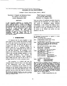
This section is devoted to study the phenomenon of extinction concentrated in a sphere S = fjxj = r� > 0g. Such a possiblity may arise for solutions with initial data concentrated in an annulus, when the outer interface moves inwards to meet the inner one at a nite radius r� > 0. This will happen for instance in the case of a thin annulus with a big hole inside. On the contrary, when the anunulus is thick and the hole is small the inner interface will reach x = 0 very soon while the outer interface is still far away, so that the hole disappears and we get the situation of Sections 4-6. Both situations are robust. As we have said, the annular solutions of Section 5 represent a borderline case, where the two interfaces meet at x = 0, precisely at the extinction time.
t
t
t
u>0
u>0
u>0 r
single point extinction
r
r
extinction on a sphere
annular type extinction
Scheme of the three extinction types for data with annular support We state conditions under which the extinction set contains a sphere S and not the origin (Theorem 8.1), more in particular, we assume that the support of u0 (r) is an annulus, e.g., (8.1)
supp u0 = f1 < r < 2g;
and then prove that the extinction pro le and extinction rates are the same as in the one-dimensional problem, as stated in Theorem 8.2 below. The following result which is proved by comparison with stationary solutions of problem (0.1)-(0.2). Lemma 8.1. Assume that for all r 2 (1; 2) � � 2 u0(r) � min log r; 2 log r for N = 2; (8.2) n o u0(r) � N 1? 2 min 1 ? r?(N ?2) ; 2N ?1 r?(N ?2) ? 2 for N � 3: Then for all t 2 (0; T ) (8.3)
supp u(r; t) � (� (t); � (t)) � [1; 2]; 35
and hence 0 62 E:
8.1. Rescaled equation. Main result. Thus, assuming that there exists a sphere fr = r� 2 [1; 2]g in the extinction set E , we introduce the rescaled variables (cf. (4.4)) (8.4) w(�; � ) = (T ? t)?1=2u(r; t); � = (Tr??tr)�1=2 ; � = ? log(T ? t): The rescaled function w solves the following equation (8.5) w� = A(w) + e?�=2 B(w); where A is the one-dimensional operator (as in (8.1)) (8.6) A(w) = w�� ? 21 w� � + 21 w and (8.7) B(w) = r +N e??�=1 2 � w� : �
The initial function for � = �0 we denote by w0 (�). Equation (8.5) looks like an exponentially small perturbation of the one-dimensional equation (7.1). We have Theorem 8.2. Assume that (8.1) and (8.2) hold. Then there exists a unique r� > 0 such that (6.20) is valid with f0 given by (7.4). The interfaces also converge. 8.1. First bounds. A gradient bound has been proved in [CV], (8.8) jw� j � M in = S (� ) � (�0; 1); where S (� ) � supp w(�; � ) = (�(� ); (� )). In this radial case it also follows from the Maximum Principle for rN ?1 ur . As in the previous problems, (8.8) implies uniform boundedness of the solution: Lemma 8.3. w � M1 in . Proof. Assuming that for some �K > �0 K = kw(�; �K )k1 � w(�K ; �K ) � 1, we derive a contradiction for the extinction time of the corresponding solution of (0.1). Indeed, from (8.8) we conclude that (8.9) w(�; �K ) � [K ? M j� ? �K j]+ : Consider the solution u(r; t) for t = tK � T ? e?�K . It follows from (8.9) and (8.4) that h i (8.10) u(r; tK ) � (T ? tK )1=2 K ? M j(r ? r� )(T ? tK )?1=2 ? �K j + for r � 0: Therefore, we can x the explicit radial symmetric solution of the form us (x; tK ) � (T ? tK )1=2f0(jx ? xK j(T ? tK )?1=2); with an arbitrary xK 2 fjxj = rK g, rK = r� + �K (T ? tK )?1=2, and with f0 given by (5.2), such that by (8.10) (8.11) u(r; tK ) � us(x; tK ) in supp us (x; tK ): This leads to contradiction since by comparison (8.11) means that the solutions u and us cannot have the same extinction time, see the proof of Proposition 4.1. � We now show that the limit pro le is concave. 36
Lemma 8.4. We have w�� � M2e?�=2 in :
(8.12)
Proof. The function z = �u � urr + ((N ? 1)=r)ur satis es in the heat equation zt = �z. Using the identities similar to (7.10) we have that on the right interface r = � (t) of the solution u(r; t) instead of (7.11) there holds (8.13) zr = ?zurr � ?z2 ? N �? 1 z � ? N �? 1 z: Similarly, on the left interface r = � (t) �
�
(8.14) zr = z z ? N �? 1 � 0 if z � (N ? 1)=�: Since by Lemma 8.1 � 2 [1; 2], we have that zr � 0 at r = � provided that z � N ? 1. Finally, from (8.13), (8.14) by the Maximum Principle we conclude that z � M 0 = max fsup �u0 ; N ? 1g in . Since jur j � M , we have for all r 2 (� (t); � (t)) urr � M 0 ? N r? 1 ur � M3: Hence, (8.12) follows by the scaling transformation (8.4). � 8.3. Mass equation. We now estimate the mass function (8.15)
E (� ) =
Z
(� )
�(� )
w(�; � ) d�:
>From the support bounds (8.3) and the w estimate (Lemma 8.3) we get a rst estimate (8.16)
E (� ) = O(e�=2):
Integrating equation (8.5) over S (� ) = (�(� ); (� )) we arrive at the mass equation Z dE ? �= 2 B(w)(� )d�: (8.17) d� = E (� ) ? 2 + e Now, we have Z Z w ? �= 2 ?�=2 B(w)d� = (N ? 1) e (r� + �e?�=2 )2 d� = O(e )E (� ): and hence (8.17) becomes dE = E (� )[1 + O(e?� )] ? 2 for � � 1; (8.18) d� 37
Lemma 8.5. As � ! 1 we have (8.19)
E (� ) = 2 + O(e?� ):
Proof. If E is larger than the estimate (8.19) the trajectory will go up to 1 with a growth of the form E (� ) � O(e� ), against (8.16). On the other hand, if the bound is violated from below the function E will reach the value 0 for a nite � . against the de nition of the rescaled time � . � With these preliminaries the estimate of Lemma 7.3 is also valid. 8.4. Bounds on interfaces. Lemma 8.6. There holds (8.20)
(� ) � M for � > �0:
Proof. We argue as in the proof of Lemma 7.4. Assume that there exists �2 � 1 such that (�2) � 1: Consider rst the case when �(� ) > c > 0 for arbitrarily larger times. From the interface equation we obtain for the left interface �0 = ?w� � ?w�� + 21 � ? e?�=2 r +N e??�=1 2 � ; � and hence by (8.12) (8.21)
�0 � 21 � ? M 0 e?�=2 for � > �2 � 1:
Integrating over (�2; � ) we deduce that (8.22)
�(� ) � �(�2 )e(� ?�2 )=2(1 + o(1)) as � ! 1:
It then follows from (8.4) that the left interface in the original spatial variable r satis es (8.23)
� (t) � r� + �(�2 )e?�2 =2(1 + o(1)) for t � T;
which indeed contradicts the de nition of r = r� as the extinction point, r� 2 E . In the second case when � is bounded and negative we apply a mass analysis. Namely, under the same hypotheses as in the proof of Lemma 7.4 by integrating equation (8.5) over (�(� ); l) we arrive at estimate (7.31) with an extra term in the right-hand side: (8.24)
@ Z l w(� )d� � ?1 + e?�=2 Z l B(w(� ))d�: @� �(� ) �(� ) 38
Integrating by parts in the last term(we obtain ) Z l Z l w w ( l; � ) e?�=2 B(w) = (N ? 1)e?�=2 r + e?�=2 l + e?�=2 (r + e?�=2 �)2 ! 0: � � � � The rest of the proof is the same as in (7.30)-(7.32). The remaining case is similar. � >From the above results, (7.33) and (7.34) follow. 8.5. Approximate Lyapunov function. Since equation (8.5) is not autonomous in time, it does not admit an explicit Lyapunov function like (7.35). Nevertheless, it is an approximate Lyapunov function and the following estimate holds. Lemma 8.7. We have ! 1
Z
(8.25)
(� )
Z
�(w� )2 d� < 1:
�(� )
�0
Proof. Multiplying equation (8.5) by �w� and integrating over S � (�1; �2) with xed �1 � 1 and an arbitrary �2 > �1 yield ! Z
�2
�1
Z
�
�(w�
= L[w](�1) ? L[w](�2) +
)2
Using an obvious estimate in the last term Z
�
�B(w)w� � M j
�M we obtain that
Z
�
�(w� )2 Z
�2 �1
Z
�
�2
Z
�1
�w� w� j � M
!1=2
�M 1+
e?�=2
Z
Z
�
�
Z
�
�B(w)w� :
p�jw j � !
�(w� )2 ;
!
Z
�
�(w� )2 � M;
where the constant M does not depend on �2 that yields the result.
�
As in the proof of Lemma 6.4, by passing to the limit in equation (8.5) we establish that the !-limit set, !(w0), consists of nontrivial bounded pro les ff g satisfying the limit stationary equation (8.26) A(f ) = 0; with A given in (8.6). It follows from the mass estimate (8.19) that for any f 2 !(w0 ) Z (8.27) f d� = 2; and (8.12) implies (8.28) f 00 � 0: The rest of the proof of Theorem 8.2 is very similar to the end of proof of Theorem 7.1.
�
39
9. Focusing at the origin
We end our present investigation with a di�erent singular phenomenon, namely the behaviour of a solution focusing at the origin in a nite time. By this we mean that the solution support (corresponding to the fresh zone) contains a hole where u = 0 and the support expands to ll this hole in nite time, the question being to describe the pro le of the solution when it approaches the focusing and the rate of convergence to such a pro le. The problem has no di�culty in one dimension because both components of the support, to the left and to the right of the hole, behave independently until they meet, and the interface behaves linearly near t = T . Therefore, we take N � 2. As in previous chapters there is a self-similar model for the focusing phenomenon, given here by formula (9.2). In particular, the interface behaviour as t ! T will be quadratic, cf. formula (9.5). Let N � 2 and let u0 (r) be a smooth, bounded function satisfying
u0 > 0; u00 > 0 on (1; 1); u0 (1) = 0; ju00j � M; ju000 j � M: Then, there exists a unique solution u(r; t) of the radially symmetric problem with initial data u0. Such a proof o�ers no di�culties with respect to what has been proved in Sections 1-3 and we will not give more details at this point. Under suitable growth conditions on u0 the solution will exist globally, moreover it exhibits nite time focusing: there exists T = T (u0) > 0 such that the unique interface r = � (t) reaches the origin lim inf � (t) = 0 and � (t) > 0 for t < T: t!T
(9.1)
The model example for such behaviour is given by the self-similar solution
u1 (r; t; T ) = (T ? t)1=2[f1(r=(T ? t)1=2)]+: with pro le f1(�) constructed in Section 5 and parameter T > 0. If we add the condition (9.3) u0 (x) � u1 (x; 0; T ) for some T > 0: then a simple comparison shows that the solution will ll its hole in a nite time and then it becomes positive everywhere (thus, a standard caloric function) for t > T , so that it exists globally in time. We can establish the following focusing description. Theorem 9.1. Let (9.1) and (9.3) be valid and T be the nite focusing time. Then as t ! T? (9.4) w(�; t) � (T ? t)?1=2u(�(T ? t)1=2; t) ! [f1(�)]+ uniformly on compact subsets in �. The interface also converges, (9.5) � (t) = �1 (T ? t)1=2(1 + o(1)) as t ! T ? ; where �1 = �1 (N ) > 0 is the unique vanishing point of the function f1 (�). Let us remark that the selection of a unique pattern is a typical nonlinear e�ect. In terms of the original variables Theorem 9.1 says that the solution u is given in rst approximation
(9.2)
40
near the focusing point, r = 0, t = T , by the self-similar formula (9.2). Such approximation is established in certain partial neighbourhoods of the form (9.6) Dc;" = f(r; t) : T ? " < t < T; 0 � r � c(T ? t)1=2g; i.e., near the free boundary. This is called the inner behaviour. It leaves out the behaviour of u on the line t = T away from the singularity r = 0 (the outer behaviour). We want to prove that it agrees with the solution u1 as r ! 0, i.e., that both behaviours match as we approach the singular point. Theorem 9.2. Under the above assumptions (9.7) u(r; T ) = a1 r(1 + o(1)) as r ! 0; where a1 (N ) > 0 is the constant in the asymptotic expansion (5.4). The universal pro le f1 (�) and the corresponding constants �1 and a1 can be calculated explicitly for N = 3, when � � p 2 1 (9.8) f1(�) = 2 � ? � and �1 = 2; a1 = 12 : On the other hand, for N = 5 p � � p 1=2 4 4 3 + 2 p2 : (9.9) f1(�) = a1 � ? � ? �3 with �1 = [2(1 + 2)] ; a1 = 4(2 + 2) We have explicitly used the notation [f1]+ to recall the reader that, when considered as a solution of our problem, the positive part has to be taken in the above formulas, cf. the opening comment in Section 5. This will be implicit in the sequel. Observe that u1 takes at t = T the exact form u1 (r; T ) = a1 r. 9.1. General comment on the problem and method. Our focusing problem has
the typical features of blow-up processes for nonlinear heat equations, namely: there arises in a nite time (t ! T ? < 1) a singular behaviour around a nite point (such point is here the origin x = 0). These two nite spatio-temporal conditions make the problem both interesting and di�cult, since it is impossible to use in the analysis the usual techniques of shifting the solution in time and space in order to construct suitable barriers and to apply other standard techniques from the theory of parabolic equations. This di�culty is a typical one in blow-up problems. To avoid this, in the present paper as well as in other blow-up studies we apply the Intersection Comparison argument to construct nonstandard \barriers". Nevertheless, let us observe that in the present problem the asymptotic behaviour reduces to the study of in nite-time stabilization for an autonomous in time parabolic equation (with a free boundary), a problem which is well known in the general theory. Actually, this is a common property of focusing stated for pure parabolic operators with power-like nonlinearities. (Extra di�culties concerning the Lyapunov instability of the a priori bounds via Intersection Comparison). A very useful tool that applies in this case is the existence of a standard explicit or implicit Lyapunov function (formally, this can be done for any quasilinear autonomous parabolic equation [Z], and it is necessary to check its good properties in order to pass to the limit). 41
Therefore, in comparison with known blow-up problems where more complicated, essentially nonlinear nonautonomous equations appear in the dynamical systems are needed (see e.g. [GV1], [GV2], [GV3] and references therein), focusing problems can be fortunately solved in a rather standard way using some of the ideas developed in blow-up research. We propose here a somewhat general scheme to study focusing free-boundary problems which is expected to be useful for di�erent equations with other quasilinear di�usion operators and nonlinear lower order terms. In general, the present analysis consists of ve main steps. (i) Control of the interface (free boundary) of the rescaled function w from above and below by using suitable geometrical properties of the stationary rescaled pro les (via the Intersection Comparison technique). (ii) A semiconvexity argument. (iii) A mass equation. (iv) A standard Lyapunov analysis in passing to the limit in the rescaled equation to prove Theorem 9.1. (v) A matching procedure to continue the expansion on compact subsets in the rescaled spatial variable � to small subsets in the original variable r = jxj, Theorem 9.2. 9.2. Existence of focusing. This can be easily proved by comparison with the selfsimilar solutions with single-point extinction on an annulus of Section 5. On the other hand, it is easy to see that this can be done by comparison with subsolutions. namely, we x an arbitrary l > �0 and set u(r; t) = (T0 ? t)1=2cl f (�; l); � = (T ?r t)1=2 ; T0 > 0; (9.10) 0 where cl > 0 is chosen so that cl f 0(�� (l); l) � 1. By comparison we have Lemma 9.3. Let in addition to (9.1) (9.11)
u0 (r) � u(r; 0) for r � 1:
Then there exists focusing at the origin and T (u0 ) � T0 .
9.3. Bounds on the interface and eventual monotonicity. We now consider the rescaled equation (4.6.a) in = f� > (� )g � (�0; 1), where � = (� ) denotes the interface, with the conditions
w = 0; w� = 1 for � = (� ); � � �0; and smooth, bounded and increasing initial data w0 (�), see (9.1).
(9.12)
Lemma 9.4. There holds
(9.13)
0 < m2 � (� ) � M2 for � > �0:
Proof. It is similar to the proof of Proposition 6.1. 42
Lower bound. We x l2 � �0 ; l2 > �0 , and consider the function
f~(�; l2) = cf (�; l2);
(9.14)
where the function f is as in (5.7) - (5.9) and the constant c is such that f~0(�� ; l2) = 1. It follows from (5.10) that in the positivity domain (9.15)
f~(�; l2) ! 0 as l2 ! �0+ uniformly:
Therefore, we may suppose that the number of intersections of the functions f~(�; l2) and w0 (�) satis es I (�0; l2) � 1 (cf. (6.2)). As in (6.3) we get the lower bound in (9.13) with m2 = �� (l2) > 0 since both solutions are assumed to have the same focusing extinction time at the origin. Upper bound. Denote by f�(�; l) the solution of (5.1) for � > l with boundary conditions (cf. (5.7))
f�(l; l) = 0; f�0 (l; l) = 1:
(9.16)
It follows from (5.8) and from asymptotics (5.3) and (5.4) that for l � 1 (9.17)
f�(�; l) � 2l
"� � N +1
l �
e(� ?l =4 ? �l 2
#
2)
on [l; l + 1];
and therefore it is easy to check that (9.18)
f��0 (�; l) ! 1 as l ! 1
uniformly on any set f� > l : 0 � m � f� � M g. Hence, in view of the regularity of w0 we have that there exists l2 � 1 such that (6.2) holds, i.e., one intersection. Therefore, by comparison (� ) � l2 for all � > �0 whence the upper bound in (9.13) with M2 = l2. � 9.4. Semiconvexity. It follows from [CV] that (9.19)
jw� j � M in ;
and hence (9.20)
w(�; � ) � M (1 + �):
Using exactly the same argument as in the proof of Proposition 8.4, from (9.1) we have ur � 0 and therefore we arrive at the inequalities
urr � M 0 ? N r? 1 ur � M; 43
whence
w�� � Me?�=2 in :
(9.21)
9.5. The ! -limit set. We now introduce the ! -limit set
(9.22)
!(w0) = fg 2 C : 9 a sequence f�k g ! 1 such that w(�; �k ) ! g(�) uniformly on compact subsetsg:
Then we have from (9.19)-(9.21) that any g 2 !(w0) satis es 0 � g(�) � M (1 + �); g�� � 0:
(9.23)
9.6. Weighted mass equation. Rewriting the equation in divergence form, (6.11), and integrating it over S (� ) = f� > (� )g we arrive at the equation
d E (� ) = 1 E (� ) ? �j �= (� ); d� 2
(9.24) for the weighted mass (9.25)
Z
E (� ) = �w d� =
Z
1 (� )
w(�; � )e?�2=4�N ?1 d�:
Lemma 9.5. There holds (9.26)
0 < m3 � E (� ) � M3 for � > �0:
Proof. The upper bound follows from (9.20). To prove the lower one we assume for a moment E (�1) � 1 for some �1 > �0. Since is bounded below, (9.13), we get from (9.24) that for � > �1
E 0(� ) � 21 E (�1) ? c < 0; c = min f�(m2); �(M2)g; i.e., E (� ) vanishes in a nite time contradicting the Strong Maximum Principle. Corollary 9.6. We have separation from the trivial limit: (9.27)
�
0 62 !(w0 ):
9.7. Lyapunov analysis. Proof of Theorem 9.1. One can check that under the above hypotheses the problem admits an explicit Lyapunov function (cf. (6.13)) of the form � Z 1 � Z 1 1 1 1 2 2 (9.28) L[w](� ) = 2 � (w� ) ? 2 w + 2 �(s)ds; (� ) (� ) 44
which is nonincreasing on evolution orbits. Therefore, !(w0 ) consists of stationary pro les ff g satisfying equation (5.1) and conditions (9.23). It then follows from the properties of stationary pro les in Section 5 that (9.29)
!(w0) � f�f1(�); 0 < � � M g;
and the concavity result (9.21) implies convergence of the interface (9.30)
(� ) ! �1 as � ! 1;
which proves (9.5). It remains to prove that � = 1 in (9.29). By passing to the limit in the mass equation (9.29) we obtain that there exists the limit E (1) = 2�(�1). This means that if g = �f1 2 !(w0 ), then (9.31)
� = 2R�(�f�1) = 1: 1
Therefore, !(w0 ) = ff1 g, which completes the proof of Theorem 9.1.
�
9.8. Proof of Theorem 9.2. Matching. Since we have a precise information about the free boundary r = � (t) for t � T and u(x; t) is the solution of the heat equation in f(x; t) : 0 < t � T; jxj � � (t)g, from the linear growth rate at t = 0 we conclude that the solution exists and is locally bounded up to t = T . Indeed, estimates (9.19)-(9.21) can be rephrased as (9.32)
u(r; t) � M (T ? t + r); jur j � M;
urr � M;
uniformly in r � � (t), 0 < t < T . In order to compare this with the `inner' behaviour of Theorem 9.1 we introduce for all xed � 2 [0; T ) the rescaled functions (9.33)
v� (r; t) = "?1=2 u(r"1=2; � + "t);
where " = "(�) � (T ? �)=T > 0. It is immediate that v� is a solution of the heat equation (written in radial coordinates) in the domain f0 � t � T; r � ��(t) = "?1=2 � (� + "t)g. Rephrasing the results of previous subsections we can say that for 0 � t � T ? � < T the family converges, (9.34)
lim v (r; t) = u1 (r; t) �!T �
uniformly on compact subsets 0 � r � K . Moreover, the interfaces also converge uniformly for 0 � t � T . Now, in every domain of the form DK = f(r; t) : 0 � t � T; K � rg with K large the v� 's are a family of positive solutions of the heat equation satisfying uniformly the estimates listed in (9.32). It follows that on compact subsets of DK it converges to a limit v~ along a subsequence �n. The point here is that we allow t ! T for xed r > 0. Now, we know that on any subset away from t = T the family v� converges to u~ = u1 . We 45
conclude that the whole family v� converges to u1 and formula (9.34) is true on compact subsets of DK . We may now take a xed point (r0 ; T ) to get lim v (r ; T ) = u1 (r0; T ); �!T � 0 which is equivalent to (9.7).
Remark. After the focusing time the hole and the free boundary disappear and the solution can be naturally continued as a solution of the heat equation in the whole space. The behaviour at r � 0 for t > T , t � T , is easily shown to be self-similar with (9.35)
u(0; t) � c2 (t ? T )1=2:
Acknowledgments
This paper was written during visits of the rst and the third authors to the Mathematical Institute, University of Leiden, and the second author to the Department of Mathematics, University Aut�onoma of Madrid. We are deeply grateful to both institutions for their hospitality. At that time the rst author was a professor of Keldysh Institute of Applied Mathematics, Moscow, and a visiting professor at University Aut�onoma, Madrid. We also want to thank A. M. Meirmanov for having brought to our attention the early work of V.A. Florin and T.D. Ventsel'. The work has been partially supported by EEC Grant SC1-0019-C(TT) and DGICYT Project PB90-0218 (Spain).
References
[AG] D. Andreucci and R. Gianni, Classical solutions to a multidimensional free boundary problem arising in combustion theory, Comm. Partial Di�er. Equat. 19 (1994), 803-826. [Am] H. Amann, Quasilinear evolution equations and parabolic systems, Trans. Amer. Math. Soc. 293 (1986), 191-227. [A1] S. Angenent, The zero set of a solution of a parabolic equation, J. Reine Angew. Math. 390 (1988), 79-96. [A2] S. Angenent, Solutions of the one-dimensional porous medium equation are determined by their free boundary, J. London Math. Soc. 42 (1990), 339-353. [A3] S. Angenent, Nonlinear analytic semi ows, Proc. Royal Soc. Edinburgh 115A (1990), 91-107. [AA] S. Angenent and D.G. Aronson, The focusing problem for the radially symmetric porous medium equation, Comm. Partial Di�er. Equat. 20 (1995), 1217-1240. [AG] D.G. Aronson and J. Graveleau, A selfsimilar solution to the focusing problem for the porous medium equation, European J. Appl. Math. 4 (1993), 65-81. 46
[B] [BCN] [BNS] [BHS] [BLS] [BL] [C] [CV] [Fl] [FK] [Fr] [GKS] [GV1] [GV2] [GV3] [HH1]
G.I. Barenblatt, "Similarity, self-similarity and intermediate asymptotics", Consultants Bureau, New York, 1968. H. Berestycki, L.A. Ca�arelli and L. Nirenberg, Uniform estimates for regularization of free boundary problems, In: \Analysis and Partial Di�erential Equations", Marcel Dekker, New York, 1990. H. Berestycki, B. Nicolaenko and B. Scheurer, Travelling waves solutions to combustion models and their singular limits, SIAM J. Math. Anal. 16 (1985), 12071242. M. Bertsch, D. Hilhorst and C. Schmidt-Lain�e, The well-posedness of a freeboundary problem arising in combustion theory, Nonlinear Anal., Theory, Meth. Appl. 23 (1994), 1211-1224. C.M. Brauner, A. Lunardi and Cl. Schmidt-Lain�e, Stability of travelling waves with interface conditions, Nonlinear Anal., Theory, Meth. Appl. 19 (1992), 455-474. J.D. Buckmaster and G.S.S. Ludford, \Theory of Laminar Flames", Cambridge University Press, Cambridge, 1982. L.A. Ca�arelli, A monotonicity formula for heat functions in disjoint domains, In: \Boundary Value Problems for PDE's and Applications", dedicated to E. Magenes, J.L. Lions, C. Baiocchi Eds, Masson, Paris, 1993, pp. 53-60. L.A. Ca�arelli and J.L. Vazquez, A free boundary problem for the heat equation arising in ame propagation, Trans. Amer. Math. Soc. 347 (1995), 411-441. V.A. Florin, Earth compaction and seepage with variable porosity, taking into account the in uence of bound water, Izvestiya Akad. Nauk SSSR, Otdel. Tekhn. Nauk, No. 11 (1951), 1625-1649 (in Russian). D.A. Frank-Kamenetskii, \Di�usion and Heat Exchange in Chemical Kinetics", Princeton Univ. Press, Princeton, 1955. A. Friedman, On the regularity of the solutions of non-linear elliptic and parabolic systems of partial di�erential equations, J. Math. Mech. 7 (1958), 43-59. V.A. Galaktionov, S.P. Kurdyumov, and A.A. Samarskii, On asymptotic "eigenfunctions" of the Cauchy problem for a nonlinear parabolic equation, Matem. Sbornik 126 (1985), 435-472 (in Russian); English translation: Mathem. USSR Sbornik 54 (1986), 421-455. V.A. Galaktionov and J.L. Vazquez, Regional blow-up in a semilinear heat equation with convergence to a Hamilton-Jacobi equation, SIAM J. Math. Anal. 24 (1993), 1254-1276. V.A. Galaktionov and J.L. Vazquez, Extinction for a quasilinear heat equation with absorption I. Technique of intersection comparison, Comm. Partial Di�er. Equat. 19 (1994), 1075-1106. V.A. Galaktionov and J.L. Vazquez, Geometrical properties of the solutions of one-dimensional nonlinear parabolic equations, Math. Ann., 1995, to appear. D. Hilhorst and J. Hulshof, An elliptic-parabolic problem in combustion theory: convergence to travelling waves, Nonlinear Anal., Theory, Meth. Appl. 17 (1991), 519-546. 47
[HH2] D. Hilhorst and J. Hulshof, A free boundary focusing problem, Proc. Amer. Math. Soc. 121 (1994), 1193-1202. [H1] J. Hulshof, An elliptic-parabolic free boundary problem: continuity of the interface, Proc. Roy. Soc. Edinburgh 106A (1987), 327-339. [H2] J. Hulshof, Spherically symmetric solutions of an elliptic-parabolic Neumann problem, Rocky Mountain Math. J. 21 (1991), 671-681. [M] A.M. Meirmanov, On a free boundary problem for parabolic equations, Matem. Sbornik 115 (1981), 532-543 (in Russian); English translation: Math. USSR Sbornik 43 (1982), 473-484. [N] K. Nickel, Gestaltaussagen uber Losungen parabolischer Di�erenzialgleichungen, J. Reine Angew. Math. 211 (1962), 78-94. [S4] A.A. Samarskii, V.A. Galaktionov, S.P. Kurdyumov, and A.P. Mikhailov, Blowup in Quasilinear Parabolic Equations, Nauka, Moscow, 1987 (in Russian); English translation: Walter de Gruyter, 19, Berlin/New York, 1995. [S] D.H. Sattinger, On the total variation of solutions of parabolic equations, Math. Ann. 183 (1969), 78-92. [St] C. Sturm, M�emoire sur une classe d'�equations �a di��erences partielles, J. Math. Pure Appl. 1 (1836), 373-444. [V1] J.L. Vazquez, Singular solutions and asymptotic behaviour of nonlinear parabolic equations, in \International Conference on Di�erential Equations; Barcelona 91", C. Perell�o, C. Sim�o and J. Sol�a-Morales eds., World Scienti c, Singapore, 1993. Pp. 234-249. [V2] J.L. Vazquez, The free boundary problem for the heat equation with xed gradient condition, to appear in Proceedings of the Conference \Free boundary problems: theory and applications", Zakopane, Poland, June 1995. [Ve] T.D. Ventsel', A free boundary-value problem for the heat equation, Dokl. Akad. Nauk SSSR 131 (1960), 1000-1003; English transl. Soviet Math. Dokl. 1 (1960). [W] F.A. Williams, \Combustion Theory", 2nd. ed., Benjamin Cummnings, 1985. [ZFK] Ya.B. Zeldovich, D.A. Frank-Kamenetski, The theory of thermal propagation of
ame, Zh. Fiz. Khim. 12 (1938), 100-105 (in Russian; english translation in \Collected Works of Ya. B. Zeldovich", vol. 1, Princeton Univ. Press, 1992). [Z] T.I. Zelenyak, Stabilization of solutions of boundary value problems for a secondorder parabolic equation with one space variable, Di�erentsial'nye Uravneniya 4 (1968), 34-45; English translation: Di�er. Equat., 4 (1968).
48