Abstract. We present a method for avoiding cracks in isosurfaces extracted from adaptive mesh refinement (AMR) data. By combining several rectilinear grids of ...
Extracting Geometrically Continuous Isosurfaces from Adaptive Mesh Refinement Data David C. Fang1, Gunther H. Weber1, Henry R. Childs2, Eric S. Brugger2, Bernd Hamann1, and Kenneth I. Joy1 1
Center for Image Processing and Integrated Computing (CIPIC) Department of Computer Science University of California, Davis Davis, CA 95616-8562, U.S.A {fangd, weber, hamann, joy}@cs.ucdavis.edu
2
B Division Lawrence Livermore National Laboratory (LLNL) 7000 East Ave., Livermore, CA 94550, U.S.A {childs3, brugger1}@llnl.gov
Abstract We present a method for avoiding cracks in isosurfaces extracted from adaptive mesh refinement (AMR) data. By combining several rectilinear grids of different resolution, AMR methods substantially reduce storage and computation requirements to accurately represent and simulate complicated data and phenomena. AMR data consist of grids of different resolution. As a result discontinuities ("hanging nodes") arise in dependent field variables at the interfaces of different-resolution mesh elements. These discontinuities can result in “cracks” in isosurfaces extracted for a specific value of a dependent scalar variable. We describe a method for creating "transition regions" between grids of different resolution. These regions are composed of pyramid elements that allow us to avoid crack formation during isosurface extraction.
1.
Introduction
Many scientific visualization techniques, including the marching cubes3 method, operate by processing all the data throughout the domain of a simulated or experimentally acquired dataset. Operating on each cell in a volumetric domain, even a slight increase in domain size will dramatically increase computation time. With volumetric datasets continually increasing in size, techniques have been developed to reduce computation time and storage requirements necessary to visualize data in an efficient way. A popular method is to adaptively vary the resolution of the mesh used to discretize a domain, such as AMR, proposed by Berger and Colella1, see Figure 1. AMR allows several axis-aligned rectilinear grids of different resolution to exist, organized in a hierarchical fashion. The ratio of resolution between grids of two subsequent mesh levels is known as the refinement ratio. The idea behind AMR is to allow the resolution within a mesh to change throughout the data domain to adapt to the behavior of the underlying geometry and/or physical phenomenon. Regions of higher resolution allow small-scale features to be captured. The adaptivity of AMR grids allows detailed features to be preserved in a large physical domain without the need for a single high-resolution, space-consuming, uniform-sized rectilinear grid.
Figure 1: AMR grid over a 2D domain. Bold points indicate hanging nodes.
An octree is another popular data structure used for reducing the computation time needed for volume visualization. An octree supports a hierarchical tree representation of data, subdividing a given data domain into eight equal-size child regions in a refinement step. The hierarchical structure allows a visualization method to use varying cell resolutions. Octree-based grids are often highly similar to AMR-based representations. Problems can arise when extracting isosurfaces from meshes of varying resolution, such as AMR and octree data. In regions where different-resolution mesh elements come together, mesh points occur that lie on the edge or face of a cell. These points, known as “hanging nodes” can cause discontinuities, or cracks, in extracted isosurfaces, see Figure 2. Cracks occur since the hanging nodes lead to a domain decomposition that is not consistent with continuous, piecewise linear interpolation of dependent data values along grid edges. These cracks are not related to the ambiguous cases in the marching cubes algorithm addressed by Nielson et. al.4 which can cause “holes” in the extracted isosurface.
Figure 2: Crack in isosurface. We present a method for extracting a crack-free isosurface from an AMR grid with scalar values associated with mesh vertices (“vertex-centered data”). Instead of patching the isosurface after extraction, or modifying current visualization techniques, the grid itself is modified, either by modifying the underlying data structure or procedurally during isosurface extraction, to prevent hanging nodes from causing cracks in an extracted isosurface. A transitional region is created by subdividing hexahedral cells into pyramid cells to eliminate hanging nodes. The transitional region also allows for extraction of crack-free isosurfaces, including datasets containing refinement ratios greater than 2:1. The subdivision process involved in creating the transitional regions also ensures that each of the pyramid cells corresponds to only one cell from the original grid. This correspondence is an important property when individual triangles from an isosurface need to be traced back to the originating cell from the initial grid, e.g., for visual debugging.
2.
Related Work
Several methods exist for patching cracks in isosurfaces extracted from vertex-centered data. Shu et al.’s6 method patches cracks in isosurfaces by inserting polygons of the same shape as the cracks. In certain situations, however, this patching method does not produce a good isosurface. When cracks are of substantial size, patching with similar-shaped polygons produces an isosurface with notches. These notches can be visually distracting due to the abrupt change in surface normal. The ideal patch surface for this situation should gradually transition from the higher-resolution surface. A slightly more complex solution was proposed by Shekhar et al.5, whose method fixes cracks by matching the isosurface generated from the higher-resolution cells to the isosurface generated from the lower-resolution cell. The disadvantage of this approach is that the higher-resolution data are ignored in order to correspond to the lowerresolution data points, thus sacrificing available detail. Westermann et al.9 presented a similar approach, creating “triangle fans” to match the isosurface from the lower-resolution cells to the isosurface of the higher-resolution cells. However, Westermann’s approach to crack fixing has difficulty preventing cracks with dataset containing an integer refinement ratios different from 2:1. Weber et al.7, 8 proposed a solution for crack fixing for cell-centered data, where dependent field variables are associated with the center of a mesh element and not with its vertices. Their solution creates a dual grid by remeshing the data such that the cell-centered data points become vertices of a new, dual mesh. This re-meshing approach allows “stitch cells” to be inserted between grids of different resolution, eliminating hanging nodes. The dual grids and stitch cells can be created without the need for interpolation of data points, eliminating any
inconsistencies due to interpolation. The drawback of this approach is that the dimension of the dataset is reduced by a cell’s width in each coordinate direction due to re-meshing. Problems can arise, for example, when the data is part of a larger dataset that has been split for purposes of parallel processing. The re-meshing also creates cells that overlap cells of the original grid, therefore not allowing extracted isotriangles to have a single correspondence with cells from the original grid, a useful property for visual debugging.
3.
Algorithm
Generating a crack-free isosurface by means of mesh manipulation necessitates a special case treatment for all transitional regions between meshes of different resolution. The transitional regions should be composed of polyhedra that generate crack-free contours along shared edges and faces. Creating a transitional region requires us to identify boundary cells. Boundary cells are defined as cells that either share an edge or face with another cell from a different-resolution mesh. Boundary conditions can be tested via connectivity data, if provided, or by determining the existence of a vertex located in the interior of a face or of an edge. The existence of a face-interior or edge-interior point indicates that the face is shared by multiple, higher-resolution cells. Once boundary cells that are not of highest resolution are identified, subdivision begins. We first discuss the 2D case, which subdivides 2D cells to create transition regions composed of rectangles. The subdivided rectangular cells created by the 2D algorithm are then used as the base of the pyramids in the 3D case. Examples are shown for meshes with a refinement ratio that is a power of two, but our algorithm can be generalized to other refinement ratio factors.
3.1.
The 2D Case
Avoiding cracks in 2D AMR meshes requires us to ensure that all hanging nodes are either eliminated by means of subdivision of cells or interpolated in such a way that cracks do not result. A transitional mesh region is created between grids of different resolution by subdividing the boundary cells of the lower-resolution grid such that the original hanging nodes are eliminated. Examples of cell face subdivision are shown in Figure 3.
a)
b)
c)
d)
Figure 3: Four examples of cell face subdivision in 2D case. Bold points indicate hanging nodes. Dashed lines indicate newly created faces. A cell face is split when a hanging node exists on the midpoint of an edge of a cell. Cell faces can be subdivided in two ways, depending on the geometry of the face, relative to the edge begin tested. A face that is a square or that is taller than it is wide is split into three sections: First, it is split in half, parallel to the edge containing the hanging node. Next, the newly created cell adjacent to the hanging node is split to eliminate the hanging node. This operation is illustrated as case a) shown in Figure 5. If a cell face is not a square or tall, the face is split into two halves along the hanging node, as shown as case b) in Figure 5. Cases c) and d) show examples of cell subdivision for refinement ratios of 2:1 and 4:1.
Once a face is subdivided, the new faces must be tested again for hanging nodes from the original data points. If these points exist, then further subdivision is needed. Subdivision continues until all hanging nodes from the original data are eliminated. When splitting cell faces, the order used to process edges can affect the result. Thus, the processing order during refinement must remain consistent throughout the subdivision process. In our examples, cell edges are tested in a left-right-top-bottom order.
Figure 4: Example of scalar value interpolation of new vertices. Bold points indicate newly formed vertices. Arrows indicate points used for linear interpolation of the newly formed vertices. The scalar values of newly created vertices are linearly interpolated using the nearest-point values along an edge, as seen in Figure 4. Hanging nodes of the original dataset are eliminated, but hanging nodes can still exist after cell subdivision. Cracks do not occur in the 2D case when contouring since a standard marching algorithm is also based on linear interpolation. When visualizing height field data, cracks are prevented since the higherresolution piecewise surface extraction process is linearly consistent along the edges with the lower-resolution surface. Thus, any discontinuities caused by the newly created hanging nodes cannot be perceived visually as cracks.
3.2.
The 3D Case
The transitional region must be composed of polyhedra that generate crack-free isosurfaces along shared edges and common faces. Decomposition of a cell into pyramids achieves the goal of crack-free isosurface extraction. Edges shared between polyhedra are linearly interpolated using the same vertices, ensuring identical results along shared edges. Cell faces shared between cells of different resolution produce crack-free isosurfaces since the larger face is decomposed into smaller faces identical to the higher-resolution cell faces. The only faces that share just a portion of another face are the triangular faces of the pyramids. A triangular face can be subdivided into smaller triangles and still produce a contour identical to the one produced by the original triangular face – which is the case since the same linear interpolant is used for each split triangle. Rectangles, when split into two rectangles, lead to two new bilinearly interpolated regions, resulting in a piecewise contour approximation that may not be identical to any contour line part produced by the original rectangular face, shown in Figure 5.
Figure 5: Contour lines in rectangular and triangular cells before and after subdivision. Our algorithm first identifies the boundary cells of each grid for all mesh refinement levels coarser than the finest level. Once a cell is identified as a boundary cell, decomposition into pyramids is performed. All pyramids decomposing an individual cell share a common apex. Thus, each face of the cell can be treated based on the 2D case. Once the subdivision of faces is complete, each face can be connected to a common apex to form the pyramids.
Figure 6: Cell face subdivision used in 3D case to match neighboring cell resolution. The bold point indicates a hanging node from an unseen neighboring cell. The face of a lower-resolution cell must be subdivided to match the face of the higher-resolution, neighboring cells, as shown in Figure 6. Once the cell face is decomposed, each edge of the faces is examined to determine whether further splitting is necessary along an edge. If a higher-resolution cell shares only an edge with a given face, then a hanging node exists along the edge. The cell face is subdivided in a manner similar to the 2D case to eliminate the hanging node. Examples of 3D cell face subdivision are shown in Figure 7.
Figure 7: Cell face subdivision in 3D case used to eliminate hanging nodes in original dataset. The bold point indicates a hanging node from an unseen neighboring cell. Each of the six faces of a transition-region cell undergoes the above procedure, along with each newly formed face. Processing continues until face decomposition is no longer needed, which is indicated by the absence of hanging nodes from the original data along all edges of the subdivided cell faces. Eventually, each face becomes the rectangular base of a pyramid, and the center of the cell becomes the apex for each of the split pyramids, as shown in Figure 8. The apex value within a cell is computed as follows: For each pyramid decomposing the cell, the average of the four values at the corners of its base is computed and multiplied by its base area (as a weight). The weighted averages of all these pyramids are then summed. A final value is obtained by dividing this sum by the total surface area of the original cell (i.e. the sum of the areas of all boundary faces of the cell).This weighted averaging scheme allows for larger pyramids, and thus coarser-resolution subdivided cell faces, to have greater influence on the value of the apex. Smaller subdivided cell faces have less influence since their scalar values should affect a smaller locality.
Figure 8: Pyramid decomposition of a cell, with front and rear pyramids omitted. Eleven pyramids are used to decompose the left face of the subdivided cell.
4.
Results
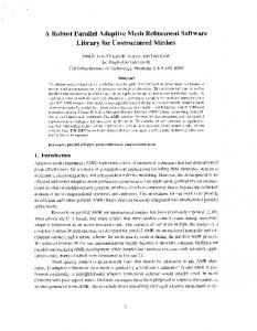
Results obtained with pyramid decomposition are provided in Table 1. Three AMR datasets were used to evaluate our technique. Tests were performed on an AMD Athlon 1.2GHz processor with 384 MB of RAM and implemented using VTK10 version 4.0.
Dataset
# cell before
# cells after
# triangles before
# triangles after
% increase in isosurface extraction time
Time (sec) to create transition regions
Test grid
17
61
3
34
N/A*
N/A*
Octree
44,332
74,358
10,456
14,332
3.85%
2.30
AMR
303,759
680,045
77,029
78,127
28.52%
7.73
Table 1: Comparisons of cell and triangle counts before and after creation of transition regions. (*Insufficient accuracy to measure) The time required to create transition regions is partially dependent on the way the multi-resolution data is stored. In our examples, no connectivity information for cells or vertices was provided, requiring 18 vertex searches (six per face and 12 per edge of a hexahedral cell) to determine whether a cell is a boundary cell. In theory, only 12 searches are needed to determine boundary conditions, but our algorithm does not take advantage of this fact. Connectivity data would speed up the creation of transition regions. It should also be noted that even though it took approximately eight seconds to process the AMR test case, this particular dataset spans a data domain of 136 × 120 × 128. It would take over two million cells using a regular rectilinear grid to span the same data domain, compared to slightly over three-hundred thousand for the AMR test grid. Thus, the additional time to create the transition regions is partially offset by the advantages of using a multiresolution data representation, such as AMR grids. Figure 9 shows an example of a large cell with 16 smaller neighboring cells, using a refinement ratio of 4:1. The decomposition into pyramids, shown on the right, leads to a significant increase in the number of cells and extracted isotriangles. The increase is apparent whenever a large refinement ratio is encountered. However, the subdivision of a larger cell into pyramids allows more accurate isotriangles to be extracted due to the higher-
resolution. It should be noted that for large datasets, the increase in cells due to the creation of a transitional region is amortized over the size of the entire dataset. Thus, the increase in the number of cells processed for isosurface extraction is dependent on the number of boundary cells found in a dataset.
Figure 9: Simple test grid decomposed into pyramids with extracted contour. Figure 10 shows results of our pyramid decomposition scheme applied to an octree grid. This particular octree was generated using a view-dependent technique2 that tends to create large continuous regions of boundary cells. Our algorithm prevents any discontinuities from occurring in the geometry of an extracted isosurface, but may produce a noticeable ridge that exists where a crack would have occurred in the original dataset, as seen in the right part of the images in Figure 10. These ridges, we believe, occur partly as a result of change in cell configuration and thus interpolation scheme, when switching from hexahedra to pyramids. There still exists ambiguity when interpolating data in transition regions. It is an open question how to properly perform scalar-value approximation in transition regions to obtain correct results in all situations, i.e., results where both geometry and function value are at least continuous.
Figure 10: Preventing cracks in an octree dataset. (Dataset courtesy of Volume Visualization System, Computer Science Department, State University of New York, Stony Brook, New York) Our method ensures that the isosurfaces extracted in transition regions are continuous in a geometrical sense and crack-free. Nevertheless, we note that hanging nodes may result on edges of extracted isotriangles due to the shared triangular faces of pyramid cells. While these hanging nodes cannot cause discontinuities in geometry, they can cause discontinuities in surface normals along an isotriangle edge. This fact can cause minor visible jumps in shading, but for typical-resolution datasets, these discontinuities are very small.
Figure 11 shows crack fixing applied to an AMR dataset. Even though the number of grid cells has doubled in this example, see Table 1, the number of extracted isosurface triangles remains similar. Unlike the octree dataset, there are no large regions of surface discontinuities that require additional triangles for crack prevention. AMR grids that are created by data-dependent methods for a specific scalar value should minimize resolution changes of cells containing the desired isosurface.
Figure 11: Preventing cracks in AMR dataset. (Dataset courtesy of Julie Coombs, Center for Neuroscience and Department of Neurobiology, Physiology, and Behavior, University of California, Davis) Due to the creation of transitional regions, single hexahedral data cells are replaced with multiple pyramid cells. The replacement scheme can noticeably increase the number of cells to process for isosurface extraction. However, it should be noted that the increase is in the number of pyramid cells. Pyramid cells are of a lower inherent polynomial degree than hexahedral cells, thus requiring less time to contour and producing relatively fewer extracted triangles than a hexahedral cell. For example, the number of cells in our AMR dataset after pyramid formation has more than doubled, but the increase in time to extract an isosurface only increases by 28.5%. Thus, the increase in the number of cells produced by our algorithm does not increase isosurface extraction time by the same magnitude as the increase in the number of cells.
5.
Conclusions and Future Work
We have presented a method for extracting and visualizing a crack-free isosurface for multi-resolution, vertexcentered AMR datasets without sacrificing inherent detail or changing the data domain. By creating transitional regions, we allow a geometrically continuous isosurface to be extracted for grids of changing resolution, including those with refinement ratios different from 2:1. The use of only hexahedral and pyramid cell elements in our crackpreventing method allows standard marching contouring algorithms to be used. All isotriangles correspond to only one cell of the original data grid, supporting visual debugging. By incorporating transitional cells into an AMR grid, isosurfaces can be extracted from a grid without fixing cracks. Our current method of face subdivision offers a compromise between the number of pyramid cells produced by the subdivision scheme and the smoothness of the extracted isosurface. By increasing the number of cells produced during cell face subdivision via a different subdivision scheme, a smoother surface should be obtained, at the cost of computation time. Producing fewer new cells during subdivision may produce a rougher isosurface, but will be computationally more efficient. It is of interest to compare different subdivision schemes to find a good balance of visual quality and computation time. Future investigation will also be directed at a different method for obtaining the scalar value of the apex of the pyramids. When used as a run-time procedural step in the isosurface extraction process, our algorithm could use a data-dependent approach to determine the apex value. A data-dependent approach would lead to a smoother isosurface.
The algorithm and examples we have presented deal with rectilinear AMR data. Our techniques can be extended to more general, curvilinear AMR data. Curvilinear datasets could be supported by creating pyramids with curved quadrilateral bases instead of planar rectangular bases.
6.
Acknowledgements
This work was supported by the Lawrence Livermore National Laboratory under ASCI ASAP Level-2 memorandum agreement B347878, and agreements B503159 and B523294; the National Science Foundation under contracts ACI 9624034 (CAREER Award), through the Large Scientific and Software Data Set Visualization (LSSDSV) program under contract ACI 9982251, through the National Partnership for Advanced Computational Infrastructure (NPACI) and a large Information Technology Research (ITR) grant; and the National Institutes of Health under contract P20 MH60975-06A2, funded by the National Institute of Mental Health and the National Science Foundation. We thank the members of the Visualization and Graphics Research Group at the Center for Image Processing and Integrated Computing (CIPIC) at the University of California, Davis, and especially Oliver Kreylos for their support and input.
7.
References
1. M. Berger and P. Colella, Local adaptive mesh refinement for shock hydrodynamics, Journal of Computational Physics, Vol. 82, pp. 64-84, May 1989. 2. D.C Fang, J.T. Grey, B. Hamann, K.I. Joy, Real-time view-dependent extraction of isosurfaces from adaptively refined octrees and tetrahedral meshes, Visualization and Data Analysis 2003, 2003 3. W.E. Lorensen, H.E. Cline, Marching cubes: A high resolution 3D surface construction algorithm, ACM SIGGRAPH Computer Graphics, Vol. 21, No. 4, pp. 163-169, July 1987 4. G.M. Nielson and B. Hamann, The asymptotic decider: resolving the ambiguity in marching cubes, IEEE in Proceedings of Visualization 91 (G.M. Nielson and L. Rosenblum, eds.), pp. 83-91, 1991 5. R. Shekhar, E. Fayyad, R. Yagel, J.F. Cornhill, Octree-based decimation of marching cubes surfaces, IEEE in Visualization, pp. 335-344, 1996 6. R. Shu, C. Zhou, M.S. Kankanhalli, Adaptive marching cubes, The Visual Computer, Vol. 11, No. 4, pp. 202217, 1995 7. G.H. Weber, O. Kreylos, T.J. Ligocki, J.M. Shalf, H. Hagen, B. Hamann, K.I. Joy, Extraction of crack-free isosurfaces from adaptive mesh refinement data, Approximation and Geometrical Methods for Scientific Visualization, pp. 19-40, 2003 8. G.H. Weber, O. Kreylos, T.J. Ligocki, J.M. Shalf, H. Hagen, B. Hamann, K.I. Joy, K. Ma, High-Quality Volume Rendering of Adaptive Mesh Refinement Data, Vision, Modeling, and Visualization 2001, pp. 121-128, 2001 9. R. Westermann, L. Kobbelt, T. Ertl, Real-time exploration of regular volume data by adaptive reconstruction of isosurfaces, The Visual Computer, Vol. 15, No. 2, pp. 100-111, 1999 10. http://www.vtk.org/