Machine Learning, 32, 101–126 (1998)
c 1998 Kluwer Academic Publishers, Boston. Manufactured in The Netherlands. °
Extracting Hidden Context MICHAEL BONNELL HARRIES
[email protected]
[email protected] Department of Artificial Intelligence, School of Computer Science and Engineering, University of NSW, Sydney, 2052, Australia
CLAUDE SAMMUT
KIM HORN
[email protected]
RMB Australia Limited, Level 5 Underwood House, 37-47 Pitt Street, Sydney, 2000, Australia Editors: Gerhard Widmer and Miroslav Kubat Abstract. Concept drift due to hidden changes in context complicates learning in many domains including financial prediction, medical diagnosis, and communication network performance. Existing machine learning approaches to this problem use an incremental learning, on-line paradigm. Batch, off-line learners tend to be ineffective in domains with hidden changes in context as they assume that the training set is homogeneous. An off-line, meta-learning approach for the identification of hidden context is presented. The new approach uses an existing batch learner and the process of contextual clustering to identify stable hidden contexts and the associated context specific, locally stable concepts. The approach is broadly applicable to the extraction of context reflected in time and spatial attributes. Several algorithms for the approach are presented and evaluated. A successful application of the approach to a complex flight simulator control task is also presented. Keywords: hidden context, concept drift, batch learning, contextual clustering, context-sensitive learning
1.
Introduction
In real world machine learning problems, there can be important properties of the domain that are hidden from view. Furthermore, these hidden properties may change over time. Machine learning tools applied to such domains must not only be able to produce classifiers from the available data, but must be able to detect the effect of changes in the hidden properties. For example, in finance, a successful stock buying strategy can change dramatically in response to interest rate changes, world events, or with the season. As a result, concepts learned at one time can subsequently become inaccurate. This concept drift occurs with changes in the context that surrounds the observations. Hidden changes in context cause problems for any machine learning approach that assumes concept stability. In many domains, hidden contexts can be expected to recur. These domains include: financial prediction, dynamic control and other commercial data mining applications. Recurring contexts may be due to cyclic phenomena, such as seasons of the year or may be associated with irregular phenomena, such as inflation rates or market mood. Machine learning systems applied in domains with hidden changes in context have tended to be incremental or on-line systems, where the concept definition is updated as new labeled observations are processed (Schlimmer & Granger, 1986). Adaptation to new domains is generally achieved by decaying the importance of older instances. Widmer and Kubat’s on-line system, Flora3 (Widmer & Kubat, 1993), exploits recurring hidden context. As the system traverses the sequence of input data, it stores concept descriptions that appear
102
M.B. HARRIES, C. SAMMUT AND K. HORN
to be stable over some interval of time. These stable concepts can be retrieved allowing the algorithm to adapt quickly when the observed domain changes to a context previously encountered. Stable concepts can also be identified off-line using batch learning algorithms. Financial institutions, manufacturing facilities, government departments, etc., all store large amounts of historical data. Such data can be analyzed, off-line, to discover regularities. Patterns in the data, however, may be affected by changes of context, where records of the context have not been maintained. To handle these situations, the batch learner must be augmented to detect hidden changes in context. Missing context is often reflected in the temporal proximity of events. For example, there may be days in which all customers buy chocolates. The hidden context in this case might be that a public holiday is due in the following week. Hidden context can also be distributed over a non-temporal dimension, making it invisible to on-line learners. For example, in remote sensing, the task of learning to classify trees by species may be affected by the surrounding forest type. If the forest type is not available to the learning system, it forms a hidden context, distributed by geographic region rather than time. Off-line methods for finding stable concepts can be applied to these domains. For simplicity, this article retains the convention of organizing hidden context over time but the methods presented generalize to properties other than time. Each stable concept is associated with one or more intervals in time. The shift from one stable concept to another represents a change in context. Thus each interval can be identified with a particular context. This presents the opportunity to build models of the hidden context. Such a model may be desirable to help understand the domain, or may be incorporated into an on-line predictive model. A model may also be used to identify a new attribute that correlates with the hidden context. In this paper, we present Splice, an off-line meta-learning system for context-sensitive learning. Splice is designed to identify stable concepts during supervised learning in domains with hidden changes in context. We begin by reviewing related work on machine learning in context-sensitive domains. This is followed by a description of the Splice methodology. An initial implementation of Splice, Splice-1, was previously shown to improve on a standard induction method in simple domains. We briefly discuss this work before presenting an improved algorithm, Splice-2. Splice-2 is shown to be superior to Splice-1 in more complex domains. The Splice-2 evaluation concludes with an application to a complex control task. 2.
Background
On-line learning methods for domains with hidden changes in context adapt to new contexts by decaying the importance of older instances. Stagger (Schlimmer and Granger, 1986), was the first reported machine learning system that dealt with hidden changes in context. This system dealt with changes in context by discarding any concepts that fell below a threshold accuracy. Splice is most related to the Flora (Widmer & Kubat, 1996) family of on-line learners. These adapt to hidden changes in context by updating the current concept to match a window of recent instances. Rapid adaptation to changes in context is assured by altering
EXTRACTING HIDDEN CONTEXT
103
the window size in response to shifts in prediction accuracy and concept complexity. One version, Flora3, (Widmer & Kubat, 1993) adapts to domains with recurring hidden context by storing stable concept descriptions, these can be re-used whenever context change is suspected. When a concept description is re-used, it is first updated to match examples in the current window. This allows Flora3 to deal with discrepancies between the recalled concept and the actual situation. Rather than an adjunct to on-line learning, Splice makes the strategy of storing stable concepts the primary focus of an off-line learning approach. Machine learning with an explicit window of recent instances, as used in Flora, was first presented by Kubat (1989) and has been used in many other on-line systems dealing with hidden changes in context. The approach has been used for supervised learning (Kubat & Widmer, 1995), and unsupervised learning (Kilander & Jansson, 1993). It is also used to adapt batch learners for on-line learning tasks by repeatedly learning from a window of recent instances (Harries & Horn, 1995; Clearwater, Cheng, & Hirsh, 1989). The use of a window can also be made sensitive to changes in the distribution of instances. Salganicoff (1993) replaces the first in, first out updating method by discarding older examples only when a new example appears in a similar region of attribute space. Most batch machine learning methods assume that the training examples are independent and unordered. As a result, batch learners generally treat hidden changes in context as noise. For example, Sammut, Hurst, Kedzier & Michie (1992), report on learning to pilot an aircraft in a flight simulator. They note that a successful flight could not be achieved without explicitly dividing the flight into stages. In this case, there were known changes of context, allowing learning to be broken into several sub-tasks. Within each stage of the flight, the control strategy, that is, the concept to be learned, was stable. Splice applies the assumption that concepts are likely to be stable for some period of time to the problem of detecting stable concepts and extracting hidden context. 3.
SPLICE
Splice’s input is a sequence of training examples, each consisting of a feature vector and a known classification. The data are ordered over time and may contain hidden changes of context. From this data, Splice attempts to learn a set of stable concepts, each associated with a different hidden context. Since contexts can recur, several disjoint intervals of the data set may be associated with the same concept. On-line learners for domains with hidden context assume that a concept will be stable over some interval of time. Splice also uses this assumption for batch learning. Hence, sequences of examples in the data set are combined into intervals if they appear to belong to the same context. Splice then attempts to cluster similar intervals by applying the notion that similarity of context is reflected by the degree to which intervals are well classified by the same concept. This is called contextual clustering. Informally, a stable concept is an expression that holds true for some period of time. One difficulty in finding a stable concept is in determining how long “some period” should be. Clearly, many concepts may be true for very short periods. Splice uses a heuristic to divide the data stream into a minimal number of partitions (contextual clusters), which may contain disjoint intervals of the dataset, so that a stable concept created from one contextual cluster will poorly classify examples in all other contextual clusters.
104
M.B. HARRIES, C. SAMMUT AND K. HORN
A more rigorous method for selecting contextual clusters might use a Minimum Description Length (MDL) measure (Rissanen, 1983). The MDL principle states that the best theory for a given concept should minimize the amount of information that needs be sent from a sender to a receiver so that the receiver can correctly classify examples in a shared dataset. In this case, the information to be sent would include stable concepts, a context switching method and a list of exceptions. A good set of contextual clusters should result in stable concepts that give a shorter description length for describing the data than would a single concept. Indeed, a possible criteria for an optimal set of contextual clusters is to achieve the minimum description length possible. A brute force approach to finding a set of clusters that minimize the MDL measure would be to consider each of the 2n possible contextual clusters in the dataset, then select a combination that covers the training set with minimum description length. Clearly, this is impractical. Splice instead uses a heuristic approach to find stable concepts that are “good enough”. The Splice algorithm is a meta-learning algorithm. Concepts are not induced directly, but by application of an existing batch leaner. In this study, we use Quinlan’s C4.5 (Quinlan, 1993), but the Splice methodology could be implemented using other propositional learning systems. C4.5 is used without modification. Furthermore, since noise is dealt with by C4.5, Splice contains no explicit noise handling mechanism. Unusual levels of noise are dealt with by altering the C4.5 parameters. The main purpose of this paper is to present the Splice-2 algorithm. However, we first briefly describe its predecessor, Splice-1 (Harries & Horn, in press) and its shortcomings to motivate the development of the Splice-2 algorithm. 3.1.
SPLICE-1
Splice-1 first uses a heuristic to identify likely context boundaries. Once the data has been partitioned on these boundaries, the partitions are combined according to their similarity of context. Stable concepts are then induced from the resulting contextual clusters. Details of the Splice-1 algorithm have previously been reported by Harries & Horn (in press) so we only give a brief overview in this section. To begin, each example must have an attribute that uniquely identifies its position in the sequence of training data. This special attribute may be provided with the data, such as a stock market trade time-stamped at 10:30 am Jan 4 1997, or may be an artificially generated serial number. The attribute, henceforth denoted as time, provides a continuum in which changes of context can be expressed. For example, a hidden context, interest rate, might change at time = 99. C4.5 is then used to induce a decision tree from the whole training set. Each node of the tree contains a test on an attribute. Any test on the special attribute, time, is interpreted as indicating a possible change of context. For example, Table 1 shows a simple decision tree that might be used for stock market investment. This tree includes a test on time, which suggests that a change in context may have occurred at time = 1995. Splice-1 then uses 1995 as boundary to partition the data set. We assume that each interval, induced by collecting all tests on time from the tree and placing them along the time axis, can be identified with a stable concept.
105
EXTRACTING HIDDEN CONTEXT
Table 1. Sample decision tree in a domain with hidden changes in context. Attribute X = true: Attribute X = false Time < 1995 Attribute A = Attribute A = Time >= 1995 Attribute B = Attribute B =
Don’t Buy
true: Buy false: Don’t Buy true: Buy false: Don’t Buy
stable concepts Splice Machine Learner
Training Set
time
Dynamic Concept Switching
On-line Classification
time
Figure 1. Splice on-line prediction.
If a stable concept induced from one interval accurately classifies the examples in another interval, we assume that both intervals are governed by similar contexts. The degree of accuracy provides a continuous measure of the degree of similarity. Splice-1 uses contextual similarity to group the intervals. This grouping is done interval by interval using a greedy heuristic that maximizes the size of contextual clusters for a given accuracy threshold. When adjacent intervals are combined, a larger context is identified. When discontiguous sub-sets are combined, a recurring context is identified. C4.5 is then applied again to the resulting contextual clusters to produce the final stable concepts. 3.2.
SPLICE-1 prediction
Harries & Horn (in press) have shown that Splice-1 can build more accurate classifiers than a standard induction algorithm in sample domains with hidden changes in context. We summarize these results and provide a comparison with the on-line method Flora3. In this task, Splice-1 is used to produce a set of stable concepts, which are then applied to an on-line prediction task. Figure 1 shows this process schematically. On-line classification is achieved by switching between stable concepts according to the current context.
106
M.B. HARRIES, C. SAMMUT AND K. HORN
3.2.1. STAGGER data set The data sets in the following experiments are based on those used to evaluate Stagger (Schlimmer & Granger, 1986) and subsequently used to evaluate Flora (Widmer & Kubat, 1996). While our approach is substantially different, use of the same data set allows some comparison of results. A program was used to generate data sets. This allows us to control the recurrence of contexts and other factors such as noise1 and duration of contexts. Each example has four attributes, size, color, shape, and time. Size has three possible values: small, medium and large. Color has three possible values: red, green and blue. Shape also has three possible values: circular, triangular, and square. The program randomly generates a sequence of examples from the above attribute space. Each example is given a serial number, to represent time, and a boolean classification based upon one of three target concepts. The target concepts are: 1. (size = small) ∧ (color = red) 2. (color = green) ∨ (shape = circular) 3. (size = medium) ∨ (size = large) Artificial contexts were created by fixing the target concepts to one of the above Stagger concepts for preset intervals of the data series. 3.2.2. On-line prediction This experiment compares the accuracy of Splice-1 to C4.5 when trained on a data set containing changes in a hidden context. In order to demonstrate that the Splice approach is valid for on-line classification tasks, we show a sample prediction problem in which Splice-1 was used off-line to generate a set of stable concepts from training data. The same training data was used to generate a single concept using C4.5, again off-line. After training, the resulting concepts were applied to a simulated on-line prediction task. C4.5 provides a baseline performance for this task and was trained without the time attribute. C4.5 benefits from the omission of this attribute as the values for time in the training set do not repeat in the test set. Even so, this comparison is not altogether fair on C4.5, as it was not designed for use in domains with hidden changes in context. The training set consisted of concept (1) for 50 instances, (2) for 50 instances, and (3) for 50 instances. The test set consisted of concepts (1) for 50 instances, (2) for 50 instances, (3) for 50 instances, and repeated (1) for 50 instances, (2) for 50 instances, and (3) for 50 instances. To apply the stable concepts identified by Splice for prediction, it was necessary to devise a method for selecting relevant stable concepts. This is not a trivial problem. Hence, for the purposes of this experiment we chose a simple voting method. With each new example, the classification accuracy of each stable concept over the last five examples was calculated. The most accurate concept was then used to classify the new example. Any ties in accuracy were resolved by random selection. The first case was classified by a randomly selected stable concept. Figure 2 plots how many times (as a percentage) the ith test example was classified correctly by Splice-1 and by C4.5 over 100 randomly generated training and test sets.
107
EXTRACTING HIDDEN CONTEXT
% correct
100 80 60 40 20
Splice C4.5
0 0
50
100
150 200 example number
250
300
Figure 2. On-line prediction task. Compares Splice-1 stable concepts with a single C4.5 concept.
Figure 2 shows that Splice-1 successfully identified the stable concepts from the training set and that the correct concept can be successfully selected for prediction in better than 95% of cases. The extreme dips in accuracy when contexts change are an effect of the method used to select stable concepts. C4.5 performs relatively well on concept 2 with an accuracy of approximately 70% but on concepts 1 and 3, it correctly classifies between 50% and 60% of cases. As noise increases, the performance of Splice-1 gradually declines. At 30% noise (Harries & Horn, in press), the worst result achieved by Splice-1 is an 85% classification accuracy on concept 2. C4.5, on the other hand, still classifies with approximately the same accuracy as it achieved in Figure 2. This task is similar to the on-line learning task attempted using Flora (Widmer & Kubat, 1996) and Stagger (Schlimmer & Granger, 1986). The combination of Splice-1 with a simple strategy for selection of the current stable concept is effective on a simple context sensitive prediction task. As the selection mechanism assumes that at least one of the stable concepts will be correct, Splice-1 almost immediately moves to its maximum accuracy on each new stable concept. For a similar problem, the Flora family (Widmer & Kubat, 1996) (in particular Flora3, the learner designed to exploit recurring context) appear to reach much the same level of accuracy as Splice-1, although as an on-line learning method, Flora requires some time to fully reflect changes in context. This comparison is problematic for a number of reasons. Splice-1 has the advantage of first seeing a training set containing 50 instances of each context before beginning to classify. Furthermore, the assumption that all possible contexts have been seen in the training set is correct for this task. On-line learners have the advantage of continuous feedback with an unconstrained updating of concepts. Splice-1 does have feedback, but is constrained to select only from those stable concepts learned from the training data. When Splice-1 has not learned a stable concept, there is no second chance. For more complex domains, it could be beneficial to use a combination of Splice-1 and an adaptive, on-line learner.
108
M.B. HARRIES, C. SAMMUT AND K. HORN
Table 2. The Splice-2 Algorithm.
(Input: Ordered data set, Window size parameter.) •
Stage 1: Partition Dataset –
Partition the dataset over time using either: ∗ ∗ ∗
•
4.
A preset number of random splits. C4.5 as per Splice-1. Prior domain knowledge.
–
The identified partitions form the initial contextual clusters.
–
C4.5 is applied to the initial contextual clusters to produce the initial interim concepts.
Stage 2: Contextual Clustering –
Each combination of interim concept and training example is allocated a score based upon the total accuracy of that concept in a fixed size window over time surrounding the example.
–
Cluster the training examples that share maximum scores with the same interim concept. These clusters form the new set of contextual clusters.
–
C4.5 is used to create a new set of interim concepts from the new contextual clusters.
–
Stage 2 is repeated until the interim concepts do not change or until a fixed number of iterations are completed.
–
The last iteration provides the set of stable concepts.
SPLICE-2
Splice-1 uses the assumption that splits on time resulting from a run of C4.5 will accurately reflect changes in context. This is not always true. A tree learned by C4.5 may contain spurious splits, or may omit important split points, due to C4.5’s greedy search strategy. Splice-2 was devised to reduce the reliance on initial partitioning. Like Splice-1, Splice-2 is a “meta-learner”. In these experiments we again use C4.5 (Quinlan, 1993) as the induction tool. The Splice-2 algorithm is detailed in Table 2. The two stages of the algorithm are discussed in turn. 4.1.
Stage 1: Partition dataset
Splice-2 begins by guessing an initial partitioning of the data and subsequent stages refine the initial guess. Any of three methods may be used for the initial guess:
EXTRACTING HIDDEN CONTEXT
109
•
Random partitioning. Randomly divide the data set into a fixed number of partitions.
•
Partitioning by C4.5. As used in Splice-1. All tests on time, found when C4.5 is run on the entire data set, are used to build the initial partitioning.
•
Prior Domain Knowledge. In some domains, prior knowledge is available about likely stable concepts.
We denote the version of Splice-2 using random partitioning as Splice-2R, the version using C4.5 partitioning as Splice-2C, and the version using prior domain knowledge as Splice-2P. Once the dataset has been partitioned, each interval of the dataset is stored as an initial contextual cluster. C4.5 is applied to each cluster to produce a decision tree known as an interim concept, see Figure 3. 4.2.
Stage 2: Contextual clustering
Stage 2 iteratively refines the contextual clusters generated in stage 1. With each iteration, a new set of contextual clusters is created in an attempt to better identify stable concepts in the data set. This process can also reduce the number of contextual clusters and, consequently, the number of stable concepts eventually learned. This stage proceeds by testing each interim concept for classification accuracy against all training examples. A score is computed for each pair of interim concept and training example. This score is based upon the number of correct classifications achieved by the interim concept in a window surrounding the example (see Figure 4). The window is designed to capture the notion that a context is likely to be stable for some period of time.
Figure 3. Splice-2: stage 1.
110
M.B. HARRIES, C. SAMMUT AND K. HORN
interim concept
Figure 4. Splice-2: stage 2. Using interim concept accuracy over a window to capture context.
On-line learning systems apply this notion implicitly by using a window of recent instances. Many of these systems use a fixed window size, generally chosen to be the size of the minimum context duration expected. The window in Splice has the same function as in an on-line method, namely, to identify a single context. Ideally, the window size should be dynamic, as in Flora, allowing the window to adjust for different concepts. For computational efficiency and simplicity, we chose to use a fixed sized window. The context of an example, i, can be represented by a concept that correctly classifies all examples within a window surrounding example i. At present the window size is set to 21 examples by default (ten examples before i, and ten examples after i). This window size biases contexts identified to be of more than 21 instances duration. This was considered to be the shortest context that would be valuable during on-line classification. The window size can be altered for different domains. We define Wij to be the score for concept j when applied to a window centered on example i. X
i+w/2
Wij =
Correctjm
(1)
m=i−w/2
where: ½
1 if interim concept j correctly classifies example m 0 if interim concept j misclassifies example m w = the window size
Correctjm =
The current contextual clusters, from stage one or a previous iteration of stage two, are discarded. New contextual clusters are then created for each interim concept j. Once all scores are computed, each example, i, is allocated to a contextual cluster associated with the interim concept, j, that maximizes Wij over all interim concepts. These interim concepts are then discarded. C4.5 is applied to each new contextual cluster to learn a new set of interim concepts (Figure 5). The contextual clustering process iterates until either a fixed number of repetitions is completed or until the interim concepts do not change from one iteration to the next. The last iteration of this stage provides a set of stable concepts. The final contextual clusters give the intervals of time for which different contexts are active.
111
EXTRACTING HIDDEN CONTEXT
contextual clusters’
C4.5
C4.5
C4.5
interim concepts’
Figure 5. Splice-2: stage 2. Create interim concepts.
4.2.1. Alternate weight In domains with a strong bias toward a single class, such as 90% class A and 10% class B, well represented classes can dominate the contextual clustering process. This can lead to clusters that are formed by combining contexts with similar classifications for well represented classes and quite dissimilar classification over poorly represented classes. This is problematic in domains where the correct classification of rare classes is important, as in “learning to fly” (see Section 6). For such domains, the Wij formula can be altered to give an equal importance to accuracy on all classes in a window while ignoring the relative representations of the different classes. For a given example, i, and an interim concept, j, the new Wij 0 formula sums over all possible classifications the proportion of examples with a given class correctly classified. The Wij 0 formula is: Wij 0 =
C X c=1
Pi+w/2
m=i−w/2 M atch(cm , c).Correctjm Pi+w/2 m=i−w/2 M atch(cm , c)
(2)
where: C is the number of classes cm is the class number of example m ½ M atch(a, b) = ½
1 if a = b 0 if a 6= b
1 if interim concept j correctly classifies example m 0 if interim concept j misclassifies example m w = the window size
Correctjm =
4.3.
SPLICE-2 walk through
In this section we present a walk through of the Splice-2R algorithm, using a simple dataset with recurring context. The dataset consists of randomly generated Stagger instances (see Section 3.2.1) classified according to the following pattern of context: 3 repetitions of the following structure (concept (1) for 30 instances, concept (2) for 30 instances, and concept (3) for 30 instances). No noise was applied to the dataset.
contextual cluster
112
M.B. HARRIES, C. SAMMUT AND K. HORN
4 3 2 1 0
50
100
150 example number
200
250
Figure 6. Initial contextual clusters. Created by randomly partitioning the dataset.
Splice-2R begins by randomly partitioning the dataset into four periods (both the partitioning method, and number of partitions are input parameters). Each period is labeled as an initial contextual cluster. Figure 6 shows the examples associated with each of these contextual clusters as drawn from the original dataset. C4.5 is then applied to each cluster, CCi , to induce an interim concept, ICi . Table 3 shows the induced concepts. Table 3. Initial interim concepts. IC1 no (34/7.1) IC2 Color in {red,green}: yes (70.0/27.3) Color = blue: no (27.0/11.3) IC3 Color = green: yes (9.0/1.3) Color in {red,blue}: | Size = small: no (6.0/2.3) | Size in {medium,large}: yes (14.0/7.8) IC4 Size = small: no (35.0/7.2) Size in {medium,large}: | Shape = circular: yes (26.0/8.1) | Shape in {square,triangular}: | | Color in {red,blue}: no (33.0/16.5) | | Color = green: yes (16.0/6.9)
Wij is calculated for all combinations of example, i, and interim concept, j. Table 4 shows the calculated Wij scores for a fragment of the dataset. Each figure in this table represents the total accuracy of a given interim concept, ICj , on all examples in a window (over time) surrounding a particular example, i. For instance, the interim concept, IC3 , classifies 12 examples correctly in a window surrounding example number 180. Each example, i, is then allocated to a new contextual cluster based upon the interim concept, ICj , that yielded the highest score, Wij . This is illustrated in Table 4 where the highest score in each column is italicized. At the base of the table we note the new contextual cluster to which each example is to be allocated. Each new contextual cluster
113
EXTRACTING HIDDEN CONTEXT
contextual cluster
4 3 2 1 0
50
100
150 example number
200
250
Figure 7. Contextual clusters0. Created by the first iteration of the contextual clustering process. contextual cluster
4 3 2 1 0
50
100
150 example number
200
250
Figure 8. Contextual clusters000. Created by the third and final iteration of contextual clustering.
is associated with a single interim concept. For example, interim concept IC1 gives the highest value for example 80, so that example is allocated to a new contextual cluster, CC1 0. This table implies a change of context around example 182. Table 4. Wij scores for the initial interim concepts on all examples in the training set. Interim Concepts
Example Number (i) 182 183
···
180
181
IC1 IC2 IC3 IC4
··· ··· ··· ···
9 11 12 10
10 10 11 11
11 11 10 12
Allocate to
···
CC3 0
CC3 0
CC4 0
184
185
···
12 11 9 11
13 10 8 11
14 10 8 12
··· ··· ··· ···
CC1 0
CC1 0
CC1 0
···
The new contextual clusters, CCi 0, are expected to improve on the previous clusters by better approximating the hidden contexts. Figure 7 shows the distribution of the new contextual clusters, CCi 0. From these clusters, a new set of interim concepts, ICi 0 are induced. Contextual clustering iterates until either a fixed number of repetitions is completed or until the interim concepts do not change from one iteration to the next. Figure 8 shows the contextual clusters after two more iterations of the clustering stage. Each remaining contextual cluster corresponds with a hidden context in the original training set. At this point, the final interim concepts, ICi 000, are renamed as stable concepts, SCi . Stable concept one, SC1 000 is the first target concept. Stable concept three, SC3 000, is the
114
M.B. HARRIES, C. SAMMUT AND K. HORN
third target concept. Stable concept four, SC4 000, is the second target concept. Contextual cluster two, CC2 000, did not contain any examples so was not used to induce a stable concept. 5.
Experimental comparison of SPLICE-1 and SPLICE-2
This section describes two experiments comparing the performance of Splice-2 with Splice-1. The first is a comparison of clustering performance across a range of duration and noise levels with the number of hidden changes in context fixed. The second compares the performance of the systems across a range of noise and hidden context changes with duration fixed. In these experiments performance is determined by checking if the concepts induced by a system agree with the original concepts used in generating the data. Both these experiments use Stagger data, as described in the prior experiment. However, unlike the prior experiment only training data is required as we are assessing performance against the original concepts. 5.1.
Contextual clustering: SPLICE-1 ‘vs’ SPLICE-2
This experiment was designed to compare the clustering performance of the two systems. Splice-1 has been shown to correctly induce the three Stagger concepts under a range of noise and context duration conditions (Harries & Horn, in press). This experiment complicates the task of identifying concepts by including more context changes. In order to compare the clustering stage alone, Splice-2C was used to represent Splice-2 performance. This ensured that the initial partitioning used in both versions of Splice was identical. Both versions of Splice were trained on independently generated data sets. Each data set consisted of examples classified according to the following pattern of context: 5 repetitions of the following structure (concept (1) for D instances; concept (2) for D instances; and concept (3) for D instances), where the duration D ranged from 10 to 100 and noise ranged from 0% to 30%. This gave a total of 14 context changes in each training set. Splice-2 was run with the default window size of 21. The number of iterations of contextual clustering were set at three. C4.5 was run with default parameters and with sub-setting on. The stable concepts learned by each system were then assessed for correctness against the original concepts. The results were averaged over 100 repetitions at each combination of noise and duration. They show the proportion of correct stable concept identifications found and the average number of incorrect stable concepts identified. Figure 9 shows the number of concepts correctly identified by Splice-1 and Splice-2C for a range of context durations and noise levels. The accuracy of both versions converges to the maximum number of concepts at the higher context durations for all levels of noise. Both versions show a graceful degradation of accuracy when noise is increased. Splice-2 recognizes more concepts at almost all levels of noise and concept duration. Figure 10 compares the number of incorrect concepts identified by Splice-1 and Splice-2. Both versions show a relatively stable level of performance at each level of noise. For all levels of noise, Splice-2 induces substantially fewer incorrect concepts than Splice-1. As both versions of Splice used the same initial partitioning, we conclude that the iterative refinement of contextual clusters, used by Splice-2, is responsible for the improvement
115
EXTRACTING HIDDEN CONTEXT
2.5 2 1.5 1 0.5
no noise 10% noise 20% noise 30% noise
Splice 2 concepts correctly identified
concepts correctly identified
Splice 1 3
0
3 2.5 2 1.5 1 0.5
no noise 10% noise 20% noise 30% noise
0 10 20 30 40 50 60 70 80 90 100 context duration
10 20 30 40 50 60 70 80 90 100 context duration
Figure 9. Concepts correctly identified by Splice-1 and Splice-2 when duration is changed. Splice 1
Splice 2
8
10 0% noise 10% noise 20% noise 30% noise
6 4 2 0
incorrect concepts
incorrect concepts
10
8
0% noise 10% noise 20% noise 30% noise
6 4 2 0
10 20 30 40 50 60 70 80 90 100 context duration
10 20 30 40 50 60 70 80 90 100 context duration
Figure 10. Incorrect concepts identified by Splice-1 and Splice-2.
on Splice-1. These results suggests that the Splice-2 clustering mechanism is better able to overcome the effects of frequent context changes and high levels of noise. In the next experiment we further investigate this hypothesis by fixing context duration and testing different levels of context change. 5.2.
The effect of context repetition
The previous experiment demonstrated that Splice-2 performs better than Splice-1 with a fixed number of context changes. It did not, however, provide any insight into the effects of context repetition. This experiment investigates the impact of context repetition (and the associated number of hidden changes in context) on Splice performance. Once again we use Splice-2C to ensure the same partitioning used for Splice-1. We also examine the results achieved by Splice-2R. In this experiment each system was trained on an independent set of data that consisted of the following pattern of contexts: R repetitions of the structure (concept (1) for 50 instances; concept (2) for 50 instances; concept (3) for 50 instances) where R varies from one to five.
116
M.B. HARRIES, C. SAMMUT AND K. HORN
Figure 11. Concepts correctly identified by Splice-1 and Splice-2C across a range of context repetition.
The effects of noise were also evaluated with a range of noise from 0% to 40%. Splice-2 was run with the default window size of 21 with three iterations of contextual clustering. Splice-2R used 10 random partitions. The parameters for C4.5 and the performance measure used were the same as used in the prior experiment. Figure 11 shows the number of concepts correctly induced by both Splice-1 and Splice-2C for each combination of context repetition and noise. The results indicate that both systems achieve similar levels of performance with one context repetition. Splice-2C performs far better than Splice-1 for almost all levels of repetition greater than one. Comparing the shapes of the performance graphs for each system is interesting. Splice-2C shows an increasing level of performance across almost all levels of noise with an increase in repetition (or context change). On the other hand, Splice-1 show an initial rise and subsequent decline in performance as the number of repetitions increases. The exception is at 0% noise, where both versions identify all three concepts with repetition levels of three and more. Figure 12 shows the number of correct Stagger concepts identified by Splice-2R. The results shows a rise in recognition accuracy as repetitions increase (up to the maximum of 3 concepts recognized) for all noise levels. The number of concepts recognized is similar to those in Figure 11 for Splice-2C. The similarity of results for Splice-2C and Splice-2R shows that, for this domain, C4.5 partitioning provides no benefit over the use of random partitioning for Splice-2C. The results of this experiment indicate that Splice-2C is an improvement on Splice-1 as it improves concept recognition in response to increasing levels of context repetition. The performance of Splice-1 degrades with increased levels of context changes. The inability of Splice-1 to cope with high levels of context change is probably due to a failure of the partitioning method. As the number of partitions required on time increases, the task of inducing the correct global concept becomes more difficult. As the information gain available for a given partition on time is reduced, the likelihood of erroneously selecting
EXTRACTING HIDDEN CONTEXT
117
Figure 12. Splice-2R concept identification.
another (possibly noisy) attribute upon which to partition the data set is increased. As a result, context changes on time are liable to be missed. Splice-2C is not affected by poor initial partitioning as it re-builds context boundaries at each iteration of contextual clustering. Hence, a poor initial partition has a minimal effect and the system can take advantage of increases in context examples. Splice-1 is still interesting, as it does substantially less work than Splice-2, and can be effective in domains with relatively few context changes. We anticipate that a stronger partitioning method would make Splice-1 more resilient to frequent changes in context. 6.
Applying SPLICE to the “Learning to Fly” domain
To test the Splice-2 methodology, we wished to apply it to a substantially more complex domain than the artificial data described above. We had available, data collected from flight simulation experiments used in behavioral cloning (Sammut et al., 1992). Previous work on this domain found it necessary to explicitly divide the domain into a series of individual learning tasks or stages. Splice-2 was able to induce an effective pilot for a substantial proportion of the original flight plan with no explicitly provided stages. In the following sections we briefly describe the problem domain and the application of Splice-2. 6.1.
Domain
The “Learning to Fly” experiments (Sammut et al., 1992) were intended to demonstrate that it is possible to build controllers for complex dynamic systems by recording the actions of a skilled operator in response to the current state of the system. A flight simulator was chosen as the dynamic system because it was a complex system requiring a high degree of skill to operate successfully and yet is well understood. The experimental setup was to collect data from several human subjects flying a predetermined flight plan. These data would then be input to an induction program, C4.5. The flight plan provided to the human subjects was:
118
M.B. HARRIES, C. SAMMUT AND K. HORN
1. Take off and fly to an altitude of 2,000 feet. 2. Level out and fly to a distance of 32,000 feet from the starting point 3. Turn right to a compass heading of approximately 330 degrees. 4. At a North/South distance of 42,000 feet, turn left to head back towards the runway. The turn is considered complete when the azimuth is between 140 degrees and 180 degrees. 5. Line up on the runway. 6. Descend to the runway, keeping in line. 7. Land on the runway. The log includes 15 attributes showing position and motion, and 4 control attributes. The position and motion attributes record the state of the plane, whereas the control attributes record the actions of the pilot. The position and motion attributes were: on ground, g limit, wing stall, twist, elevation, azimuth, roll speed, elevation speed, azimuth speed, airspeed, climbspeed, E/W distance, altitude, N/S distance, fuel. The control attributes were: rollers, elevator, thrust and flaps. (The rudder was not used as its implementation was unrealistic.) The values for each of the control attributes provide target classes for the induction of separate decision trees for each control attribute. These decision trees are tested by compiling the trees into the autopilot code of the simulator and then “flying” the simulator. In the original experiments, three subjects flew the above flight plan 30 times each. In all, a data set of about 90,000 records was produced. Originally, it was thought that the combined data could be submitted to the learning program. However, this proved too complex a task for the learning systems that were available. The problems were largely due to mixing data from different contexts. The first, and most critical type of context, was the pilot. Different pilots have different flying styles, so their responses to the same situation may differ. Hence, the flights were separated according to pilot. Furthermore, the actions of a particular pilot differ according to the stage of the flight. That is, the pilot adopts different strategies depending on whether he or she is turning the aircraft, climbing, landing, etc. To succeed in inducing a competent control strategy, a learning algorithm would have to be able to distinguish these different cases. Since the methods available could not do this, manual separation of the data into flight stages was required. Since the pilots were given intermediate flight goals, the division into stages was not too onerous. Not all divisions were immediately obvious. For example, initially, lining up and descending were not separated into two different stages. However, without this separation, the decision trees generated by C4.5 would miss the runway. It was not until the “line-up” stage was introduced that a successful “behavioral clone” could be produced. Until now, the stages used in behavioral cloning could only be found through human intervention which often included quite a lot of trial-and-error experimentation. The work described below suggests that flight stages can be treated as different contexts and that the Splice-2 approach can automate the separation of flight data into appropriate contexts for learning.
EXTRACTING HIDDEN CONTEXT
6.2.
119
Flying with SPLICE-2
This domain introduces an additional difficulty for Splice. Previous behavioral cloning experiments have built decision trees for each of the four actions in each of the seven stages, resulting in 28 decision trees. When flying the simulator these decision trees are switched in depending on the current stage. However, when Splice-2 is applied to the four learning tasks, viz, building a controller for elevators, another for rollers, for thrust and flaps, there is no guarantee that exactly the same context divisions will be found. This causes problems when two or more actions must be coordinated. For example, to turn the aircraft, rollers and elevators must be used together. If the contexts for these two actions do not coincide then a new roller action, say, may be commenced, but the corresponding elevator action may not start at the same time, thus causing a lack of coordination and a failure to execute the correct manoeuvre. This problem was avoided by combining rollers and elevators into a single attribute, corresponding to the stick position. Since the rollers can take one of 15 discrete values and elevators can take one of 11 discrete values, the combined attribute has 165 possible values. Of these, 97 are represented in the training set. A further problem is how to know when to switch between contexts. The original behavioral clones included hand-crafted code to accomplish this. However, Splice builds its own contexts, so an automatic means of switching is necessary. In the on-line prediction experiment reported in Section 3.2.2, the context was selected by using a voting mechanism. This mechanism relied upon immediate feedback about classification accuracy. We do not have such feedback during a flight, so we chose to learn when to switch. All examples of each stable concept were labelled with an identifier for that concept. These were input to C4.5 again, this time, to predict the context to which a state in the flight belongs, thus identifying the appropriate stable concept, which is the controller for the associated context. In designing this selection mechanism we remained with the “situation-action” paradigm that previous cloning experiments adopted so that comparisons were meaningful. We found that the original Splice-2 Wij formula, which uses only classification accuracy, did not perform well when class frequencies were wildly different. This was due to well represented classes dominating the contextual clustering process, leading to clusters with similar classification over well represented classes, and dissimilar classification over poorly represented classes. This was problematic as successful flights depend upon the correct classification of rare classes. The problem was reduced by adopting the alternative scoring method defined by Equation 2 (Section 4.2.1). In addition we adjusted the C4.5 parameters (pruning level) to ensure that these rare classes were not treated as noise. Splice-2 was also augmented to recognize domain discontinuities such as the end of one flight and the beginning of the next by altering Wij 0 such that no predictions from a flight other than the flight of example i were incorporated in any Wij 0. We have been able to successfully fly the first four stages of the flight training on data extracted from 30 flights, using only data from the first four stages. It should be noted that even with the changes in the domain (combining rollers and elevator) C4.5 is unable to make the first turn without the explicit division of the domain into stages. Figure 13 shows three flights: •
The successful Splice-2 flight on stages 1 to 4.
120
M.B. HARRIES, C. SAMMUT AND K. HORN
Figure 13. Flight comparison.
•
The best C4.5 flight.
•
A sample complete flight. The settings used in Splice-2P were:
•
C4.5 post pruning turned off (-c 100).
•
Three iterations of the clustering stage.
•
A window size of 50 instances.
•
Initial partitioning was set to four equal divisions of the first flight.
We initially investigated the use of a larger window with a random partitioning. This successfully created two contexts: one primarily concerning the first five stages of the flight and the other concerning the last two. With this number of contexts, a successful pilot could not be induced. Reducing the window size lead to more contexts, but they were less well defined and also could not fly the plane. The solution was to bias the clustering by providing an initial partitioning based on the first four stages of the flight. Further research is needed to determine if the correspondence between the number of initial partitions and the number of flight stages is accidental or if there is something more fundamental involved. Splice-2 distinguished four contextual clusters with a rough correlation to flight plan stages. Each contextual cluster contains examples from multiple stages of the training
121
EXTRACTING HIDDEN CONTEXT
Context 1 Context 2 Context 3 Context 4 Height (feet) 3000 2500 2000 1500 1000 500 0
-40000
-35000
6000 5000 4000 3000 2000 East/West (feet) 1000
-30000
-25000 -20000 North/South (feet) -15000 -10000
-5000
0 -1000
Figure 14. Distribution of the local concepts used in the successful flight. The chart shows only one in sixty time steps, this was necessary for clarity but does remove some brief context changes.
flights. Context 1 has instances from all four stages but has a better representation of instances from the first half of stage 1. Context 2 roughly corresponds with the second half of stage 1, stage 2, and part of 3. Instances in context 3 are from stage 2 onward, but primarily from stage 4. Context 4 is particularly interesting as it also corresponds primarily with stage 4, but contains less examples than context 3 for all parts of this stage. It is not surprising that the correspondence of context to stage is not complete. The original division of the flight plan into stages was for convenience of description, and the same flight could well have been divided in many different ways. In short, the Splice contexts are capturing something additional to the division of the flight into stages. Figure 14 shows the stable concept used at each instant of the Splice-2 flight. To make context changes clearly visible, the number of points plotted in Figure 14 are fewer than were actually recorded. Because of the lower resolution, not all details of the context changes are visible in this chart. Take off was handled by context 1. Climb to 2,000 feet and level out was handled by context 2. Context 3 also had occasional instances in the level out region of the flight. Context 1 again took over for straight and level flight. The right hand turn was handled by a mix of contexts 3 and 4. Subsequently flying to the North-West was handled by contexts 2 and 3 then by context 4. Initiating the left hand turn was done by context 1. The rest of the left hand turn was handled by a combination of contexts 3 and 4.
122
M.B. HARRIES, C. SAMMUT AND K. HORN
When Sammut et al. (1992) divided the flight into stages, they did so by trial and error. While the partitions found were successfully used to build behavioral clones, there is no reason to believe that their partition is unique. In fact, we expect similar kinds of behaviors to be used in different stages. For example, a behavior for straight and level flight is needed in several points during the flight as is turning left or turning right. Moreover, the same control settings might be used for different maneouvres, depending on the current state of the flight. Figure 14 shows that Splice intermixed behaviors much more than was done with the manual division of stages. Although this needs further investigation, a reasonable conjecture is that an approach like Splice can find more finely tuned control strategies than can be achieved manually. In a subsequent experiment we attempted to hand craft a “perfect” switching strategy, by associating stable concepts with each stage of the flight plan. This switching method did not successfully fly the plane. At present, the inclusion of data from further stages of the flight causes catastrophic interference between the first two stages and the last 3 stages. Splice-2 is, as yet, unable to completely distinguish these parts of the flight. However, the use of Splice-2 in synthesizing controllers for stages 1 - 4 is the first time that any automated procedure has been successful for identifying contexts in this very complex domain. The use of a decision tree to select the current context is reasonably effective. As the decision tree uses only the same attributes as the stable concepts, it has no way to refer to the past. In effect, it is flying with no short term memory. This amnesia not an issue for this work as it is a comparison with the original “Learning to Fly” project (Sammut et al., 1992) which used situation-action control. This experiment serves to demonstrate that off-line context-sensitive learning can be applied to quite complex data sets with promising results. 7.
Related work
There has been a substantial amount of work on dealing with known changes in context using batch learning methods. Much of this work is directly relevant to the challenges faced in using stable concepts for on-line prediction. Known context can be dealt with by dividing the domain by context, and inducing different classifiers for each context. At classification time, a meta-classifier can then be used to switch between classifiers according to the current context (Sammut et al., 1992; Katz, Gately & Collins, 1990). The application of stable concepts to on-line classification used in this paper (Sections 3.2.2 and 6.2) uses a similar switching approach. Unfortunately, it is not always possible to guarantee that all hidden contexts are known. New contexts might be dealt with by adapting an existing stable concept. Kubat (1996) demonstrates that knowledge embedded in a decision tree can be transfered to a new context by augmenting the decision tree with a second tier, which is then trained on the new context. The second tier provides soft matching and weights for each leaf of the original decision tree. Use of a two tiered structure was originally proposed by Michalski (1987) for dealing with flexible concepts. Pratt, Mostow, & Kamm (1991) show that knowledge from an existing neural network can be re-used to significantly increase the speed of learning in a
EXTRACTING HIDDEN CONTEXT
123
new context. These methods for the transfer of knowledge between known contexts could be used on-line to adapt stable concepts in a manner analogous to that used by Flora3. It may be possible to improve the accuracy of stable concepts by combining data from a range of contexts. Turney (1993; see also Turney & Halasz, 1993) applies contextual normalization, contextual expansion and contextual weighting to a range of domains. He demonstrates that these methods can improve classification accuracy for both instance based learning (Aha, Kibler & Albert, 1991) and multivariate regression. This could be particularly valuable for a version of Splice using instance based methods instead of C4.5. A somewhat different on-line method designed to detect and exploit context is MetaL(B) (Widmer, 1997). This system seeks contextual clues in past data, these clues are then used to trigger changes in the set of instances presented to the classifier. While the MetaL approach is quite different to that used by Splice, the overall philosophy is similar. Widmer concludes by stating that: “. . . the identification of contextual features is a first step towards naming, and thus being able to reason about, contexts.” This is one of the main goals of Splice. The result of such reasoning would be a model of the hidden context. Models describing hidden context could be applied in on-line classification systems to augment existing reactive concept switching with a pro-active component. These models could also be used to improve domain understanding. Some first steps toward building models of hidden context have been taken in this article. The “Learning to Fly” experiment (Section 6.2) used a model of hidden context, based on the types of instances expected in each context, to switch between stable concepts. To summarize, Splice begins to build a bridge between on-line methods for dealing with hidden changes in context and batch methods for dealing with known change in context. 8.
Conclusion
This article has presented a new off-line paradigm for recognizing and dealing with hidden changes in context. Hidden changes in context can occur in any domain where the prediction task is poorly understood or where context is difficult to isolate as an attribute. Most previous work with hidden changes in context has used an on-line learning approach. The new approach, Splice, uses off-line, batch, meta-learning to extract hidden context and induce the associated stable concepts. It incorporates existing machine learning systems (in this paper, C4.5 (Quinlan, 1993)). The initial implementation, Splice-1, was briefly reviewed and a new version, Splice-2, presented in full. The evaluation of the Splice approach included an on-line prediction task, a series of hidden context recognition tasks, and a complex control task. Splice-1 was the initial implementation of the Splice approach and used C4.5 to divide a data series by likely changes of context. A process called contextual clustering then grouped intervals appearing to be from the same context. This process used the semantics of concepts induced from each interval as a measure of the similarity of context. The resulting contextual clusters were used to create context specific concepts and to specify context boundaries.
124
M.B. HARRIES, C. SAMMUT AND K. HORN
Splice-2 addresses limitations of Splice-1 by permitting refinement of partition boundaries. Splice-2 clusters on the basis of individual members of the data series. Hence, context boundaries are not restricted to the boundaries found in the partitioning stage and context boundaries can be refined. Splice-2 is much more robust to the quality of the initial partitioning. Splice-2 successfully detected and dealt with hidden context in a complex control task. “Learning to Fly” is a behavioral cloning domain based upon learning an autopilot given a series of sample flights with a fixed flight plan. Previous work on this domain required the user to specify stages of the flight. Splice-2 was able to successfully fly a substantial fragment of the initial flight plan without these stages (or contexts) being specified. This is the first time that any automated procedure has been successful for identifying context in this very complex domain. A number of improvements could be made to the Splice algorithms. The partitioning method used was shown to be problematic for Splice-1 at high levels of noise and with many hidden changes in context. While the use of an existing machine learning system to provide partitioning is elegant, a better solution may be to implement a specialized method designed to deal with a large number of splits on time in potentially noisy domains. One approach to this is to augment a decision tree algorithm to allow many splits (Fayyad & Irani, 1993) on selected continuous attributes. Neither Splice-1 nor Splice-2 provide a direct comparison of the relative advantage of dividing the domain into one set of contexts over another. One comparison method that could be used is the minimum description length (MDL) heuristic (Rissanen, 1983). The MDL principle is that the best theory for a given concept will minimize the amount of information that need be sent from a sender to a receiver so that the receiver can correctly classify examples in a shared dataset. In this case, the information to be sent must contain any stable concepts, a context switching method and a list of exceptions. At the very least, this would allow the direct comparison of a given context-sensitive global concept (using stable concepts and context switching) with a context-insensitive global concept. Further, a contextual clustering method could use an MDL heuristic to guide a search through the possible context divisions. The approaches used here for selecting the current context at classification time were an on-line voting method for domains with immediate feedback and a decision tree for a domain without immediate feedback. More sophisticated approaches would use a model of the hidden context. Such a model could use knowledge about the expected context duration, order and stability. It could also incorporate other existing attributes and domain feedback. The decision tree used for context switching in the learning to fly task is a primitive implementation of such a model using only existing attributes to select the context. An exciting possibility is to use the characteristics of contexts identified by Splice to guide a search of the external world for an attribute with similar characteristics. Any such attributes could then be incorporated with the current attribute set allowing a bootstrapping of the domain representation. This could be used within the Knowledge Discovery in Databases (KDD) approach (Fayyad, Piatsky-Shapiro & Smyth, 1996) which includes the notion that analysts can reiterate the data selection and learning (data mining) tasks. Perhaps too, this method could provide a way for an automated agent to select potentially useful attributes from the outside world, with which to extend its existing domain knowledge.
EXTRACTING HIDDEN CONTEXT
125
Acknowledgments We would like to thank our editors, Gerhard Widmer and Miroslav Kubat, and the anonymous reviewers. Their suggestions led to a much improved paper. We also thank Graham Mann, John Case, and Andra Keay for reading and commenting on various drafts of this work. Michael Harries would like to acknowledge the support, encouragement, and inspiration provided by his colleagues in the Department of Artificial Intelligence at the University of NSW. Michael Harries was supported by an Australian Postgraduate Award (Industrial) generously sponsored by RMB Australia. Notes 1. In the following experiments, n% noise implies that the class was randomly selected with a probability of n%. This method for generating noise was chosen to be consistent with Widmer and Kubat (1996).
References Aha, D., Kibler, D., & Albert, M. (1991). Instance-based learning algorithms. Machine Learning, 6(1), 37–66. Clearwater, S., Cheng, T., & Hirsh, H. (1989). Incremental batch learning. Proceedings of the Sixth International Workshop on Machine Learning (pp 366–370). San Mateo, CA: Morgan Kaufmann. Fayyad, U.M. & Irani, K.B. (1993). Multi-interval discretization of continuous-valued attributes for classification learning. Proceedings of the Thirteenth International Joint Conference on Artificial Intelligence (pp 1022–1027). San Mateo, CA: Morgan Kaufmann. Fayyad, U.M., Piatsky-Shapiro, G., & Smyth, P. (1996). From data mining to knowledge discovery: An overview. In Fayyad, U.M., Piatsky-Shapiro, G., Smyth, P., & Uthurusamy, R. (Ed.), Advances in Knowledge Discovery and Data Mining. Cambridge, MA: MIT Press. Harries, M. & Horn, K. (1995). Detecting concept drift in financial time series prediction using symbolic machine learning. Proceedings of the Eighth Australian Joint Conference on Artificial Intelligence (pp 91–98). Singapore: World Scientific. Harries, M. & Horn, K. (in press). Learning stable concepts in a changing world. In G. Antoniou, A. Ghose and M. Truczszinski (Ed.), LNAI 1359: Learning and Reasoning with Complex Representations. Springer-Verlag. Katz, A.J., Gately, M.T., & Collins, D.R., C. (1990). Robust classifiers without robust features. Neural Computation, 2(4), 472–479. Kilander, F. & Jansson, C.G. (1993). COBBIT - a control procedure for COBWEB in the presence of concept drift. Proceedings of the Sixth European Conference on Machine Learning (pp 244–261). Berlin: Springer-Verlag. Kubat, M. (1989). Floating approximation in time-varying knowledge bases. Pattern Recognition Letters, 10, 223–227. Kubat, M. (1996). Second tier for decision trees. Proceedings of the Thirteenth International Conference on Machine Learning (pp. 293–301). San Francisco, CA: Morgan Kaufmann. Kubat, M. & Widmer, G. (1995). Adapting to drift in continuous domains. Proceedings of the Eighth European Conference on Machine Learning (pp. 307–310). Berlin: Springer-Verlag. Michalski, R.S. (1987). How to learn imprecise concepts: A method employing a two-tiered knowledge representation for learning. Proceedings of the Fourth International Workshop on Machine Learning (pp. 50–58). Los Altos, CA: Morgan Kaufmann. Pratt, Y.P., Mostow, J., & Kamm, C.A. (1991). Direct transfer of learned information among neural networks. Proceedings of the Ninth National Conference on Artificial Intelligence (pp. 584–589). Menlo Park, CA: AAAI Press. Quinlan, J.R. (1993). C4.5: Programs for Machine Learning. San Mateo, CA: Morgan Kaufmann.
126
M.B. HARRIES, C. SAMMUT AND K. HORN
Rissanen, J. (1983). A universal prior for integers and estimation by minimum description length. Annals of Statistics, 11(2), 416–431. Salganicoff, M. (1993). Density adaptive learning and forgetting. Proceedings of the Tenth International Conference on Machine Learning (pp. 276–283). San Mateo, CA: Morgan Kaufmann. Sammut, C., Hurst, S., Kedzier, D., & Michie, D. (1992). Learning to fly. Proceedings of the Ninth International Conference on Machine Learning (pp. 385–393). San Mateo, CA: Morgan Kaufmann. Schlimmer, J. & Granger, Jr., R. (1986). Incremental learning from noisy data. Machine Learning, 1(3), 317–354. Turney, P.D. (1993). Exploiting context when learning to classify. Proceedings of the Sixth European Conference on Machine Learning (pp. 402–407). Berlin: Springer-Verlag. Turney, P.D. & Halasz, M. (1993). Contextual normalization applied to aircraft gas turbine engine diagnosis. Journal of Applied Intelligence 3, 109–129. Widmer, G. (1997). Tracking Context Changes through Meta-Learning. Machine Learning 27(3), 259–286. Widmer, G. & Kubat, M. (1993). Effective learning in dynamic environments by explicit concept tracking. Proceedings of the Sixth European Conference on Machine Learning (pp. 227–243). Berlin: Springer-Verlag. Widmer, G. & Kubat, M. (1996). Learning in the presence of concept drift and hidden contexts. Machine Learning 23(1), 69–101. Received September 22, 1997 Accepted March 27, 1998 Final Manuscript April 7, 1998