Extracting Ultra-Scale Lattice Boltzmann Performance via Hierarchical ...

Extracting Ultra-Scale Lattice Boltzmann Performance via Hierarchical and Distributed Auto-Tuning Samuel Williams, Leonid Oliker, Jonathan Carter, John Shalf Computational Research Division, Lawrence Berkeley National Laboratory { SWWilliams, LOliker, JTCarter, JShalf } @ lbl.gov

ABSTRACT We are witnessing a rapid evolution of HPC node architectures and on-chip parallelism as power and cooling constraints limit increases in microprocessor clock speeds. In this work, we demonstrate a hierarchical approach towards effectively extracting performance for a variety of emerging multicore-based supercomputing platforms. Our examined application is a structured grid-based Lattice Boltzmann computation that simulates homogeneous isotropic turbulence in magnetohydrodynamics. First, we examine sophisticated sequential auto-tuning techniques including loop transformations, virtual vectorization, and use of ISA-specific intrinsics. Next, we present a variety of parallel optimization approaches including programming model exploration (flat MPI, MPI/OpenMP, and MPI/Pthreads), as well as data and thread decomposition strategies designed to mitigate communication bottlenecks. Finally, we evaluate the impact of our hierarchical tuning techniques using a variety of problem sizes via large-scale simulations on state-of-the-art Cray XT4, Cray XE6, and IBM BlueGene/P platforms. Results show that our unique tuning approach improves performance and energy requirements by up to 3.4× using 49,152 cores, while providing a portable optimization methodology for a variety of numerical methods on forthcoming HPC systems.

Keywords Auto-tuning, Hybrid Programming Models, OpenMP, Lattice Boltzmann, SIMD, BlueGene

1.

INTRODUCTION

The multicore revolution has resulted in a vast diversity of shared memory multicore architectures that are at the heart of high-end computing platforms. An urgent challenge for the HPC community is developing methodologies for optimizing scientific computation to effectively utilize these complex and rapidly evolving systems. One key question is appropriately addressing computation in the context of a hybrid communication infrastructure: shared memory

Permission to make digital or hard copies of all or part of this work for personal or classroom use is granted without fee provided that copies are not made or distributed for profit or commercial advantage and that copies bear this notice and the full citation on the first page. To copy otherwise, to republish, to post on servers or to redistribute to lists, requires prior specific permission and/or a fee. SC11, November 12-18, 2011, Seattle, Washington, USA Copyright 2011 ACM 978-1-4503-0771-0/11/11 ...$10.00.

within nodes and message passing between nodes. Our paper presents a hierarchical and distributed approach towards achieving performance portability on emerging supercomputers by leveraging the system’s hybrid intra- and inter-node communication capabilities. Our work explores a structured grid-based Lattice Boltzmann (LBM) computation that simulates homogeneous isotropic turbulence in magnetohydrodynamics. Although this complex application has unique requirements, its computational structure is similar to a large class of explicit numerical methods. This is the first extensive study to apply the ideas of automatic tuning (or autotuning) in a two-stage hierarchical and distributed fashion for this important class of numerical simulations. We begin by exploring sequential optimizations via the auto-tuning of several important parameters including unrolling depth, virtual vectorization length, and software prefetching distance, as well as ISA-specific SIMDization and tuning. After addressing optimized sequential performance, we next explore the challenges in a parallel architectural environment, including NUMA (non-uniform memory access), affinity, problem decomposition among processes, threading with MPI/OpenMP and MPI/Pthreads, as well as improving communication performance using message aggregation and parallelized buffer packing. Having implemented a broad set of potential optimizations, we then apply a hierarchical and distributed auto-tuner that intelligently explores a subset of the tuning dimensions (sequential optimizations in the first stage and parallel in the second) by running a small problem at a moderate concurrency of 64 nodes. Finally, having derived the optimal serial and parallel tuning parameters, we validate our methodology at scale using three state-of-the-art parallel platforms: Cray XT4, Cray XE6, and IBM BlueGene/P. Detailed analysis based on the machine architectures and LBMHD problem characteristics demonstrate that our tuning approach achieves significant and performance portable results: attaining up to a 3.4× improvement in application performance using 49,152 cores compared with a previous, highly-optimized reference implementation. Additionally, exploration of varying problem sizes and parallelization approaches provide insight into the expected limitations of next-generation exascale systems, and points to the importance of hierarchical auto-tuning to effectively leverage emerging HPC resource in a portable fashion. Finally, we quantify the energy efficiency of all three platforms before and after performance optimization.

2.

LATTICE BOLTZMANN MODELS

Variants of the Lattice Boltzmann equation have been ap-

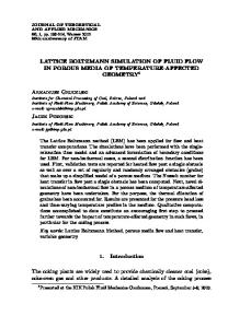
plied to problems such as fluid flows, flows in porous media, and turbulent flows over about the past 25 years [25]. Emerging from lattice gas cellular automata techniques, the model has been developed through several iterations into a mature and computationally efficient technique today. Lattice Boltzmann models that draw heavily from kinetic theory, and typically make use of a Bhatnagar-Gross-Krook [1] (BGK) inspired collision operator, have become the most common form of the technique. In this form, a simplified kinetic model is constructed that incorporates the essential physics and reproduces correct macroscopic averaged properties. Implicit in the method is a discretization of space and time (via velocities) onto a lattice, where a set of mesoscopic quantities (density, momenta, etc.) and probability distribution functions are associated with each lattice site. The probability density functions represent fluid elements at a specific time, location, and velocity as they move and collide on the lattice, and the collective behavior reflects the dynamics of fluid flow. These models may be characterized as explicit, second-order, time-stepping algorithms. Lattice Boltzmann models have grown in popularity due to their flexibility in handling complex boundary conditions via simple bounce-back formulations, and straightforward inclusion of mesoscale effects that are hard to describe with continuum approaches, such as porous media, or multiphase and reactive flows. The LBM equations break down into two separate terms, each operating on a set of distribution functions; a linear free-streaming operator and a local non-linear collision operator. The BGK inspired approximation replaces the complex integral collision operator of the exact theory by a relaxation to an equilibrium distribution function taking place on a single timescale. For the fluid dynamics case, in discretized form, we write: fa (x + ca ∆t, t + ∆t) = fa (x, t) − 1/τ (fa (x, t) − faeq (x, t)) where fa (x, t) denotes the fraction of particles at time step t moving with velocity ca , and τ the relaxation time which is related to the fluid viscosity. f eq is the local equilibrium distribution function, constructed from the macroscopic variables, the form of which is chosen to impose conservation of mass and momentum, and impose isotropy. The velocities ca arise from the basic structure of the lattice, so that a particle travels from one lattice site to another in one time step. The grid is chosen in concert with the collision operator and equilibrium distribution function. A typical 3D discretization is the D3Q27 model [37], which uses 27 distinct velocities (including zero velocity) is shown in Figure 1. Conceptually, a LBM simulation proceeds by a sequence of collision() and stream() steps, reflecting the structure of the master equation. The collision() step involves data local only to that spatial point; the macroscopic variables at each point are calculated from the distribution functions and from them the equilibrium distribution is formed. The distribution functions are then updated. This is followed by the stream() step that evolves the distribution functions along the appropriate lattice vectors. In practice however, most implementations incorporate the data movement of the stream() step directly into the collision() step—an optimization suggested by Wellein and co-workers [29]. In this formulation, either the newly calculated particle distribution function can be scattered to the correct neighbor as soon as it is calculated, or equivalently, data can be gathered from

adjacent cells to calculate the updated value for the current cell. Using this method, data movement is considerably reduced and programming the collision step begins to look much more like a stencil kernel—in that data are accessed from multiple nearby cells. A key difference is that there is no temporal reuse of grid data between the processing of one grid point and another, each variable at each grid point is used only once. In addition to conventional fluid dynamics, the Lattice Boltzmann technique has been successfully extended to the field of magnetohydrodynamics (MHD) [9, 16, 21]. MHD effects play an important role in many branches of physics [2]: from the earth’s core to astrophysical phenomena, from plasma confinement to engineering design with electrically conducting liquid metals in magnetic fusion devices. The kernel of the algorithm is similar to that of the fluid flow LBM except that the regular distribution functions are augmented by magnetic field distribution functions, and the macroscopic quantities augmented by the magnetic field. We have chosen to study the behavior of an MHD LBM code as they contain some of the more challenging kernels as compared to the fluid dynamics case. The additional macroscopic variables and distribution functions present a severe test to most compilers and memory subsystems. The LBMHD [14] code was developed using the D3Q27 lattice to study MHD homogeneous isotropic turbulence in a simple system with periodic boundary conditions. In this case, for the magnetic field distribution functions, the number of phase space velocities needed to recover information on the magnetic field is reduced from 27 to 15. The differing components for particle and magnetic field are shown in Figure 1. The original Fortran implementation of the code achieved high sustained performance on vector architectures, but a relatively low percentage of peak performance on superscalar platforms [3] The application was rewritten in C for our previous study [32], around two lattice data structures, representing the state of the system, the various distribution functions and macroscopic quantities, at time t and at time t + 1. At each time step one lattice is updated from the values contained in the other. The algorithm alternates between these each data structures as time is advanced. The lattice data structure is a collection of arrays of pointers to double precision arrays that contain a grid of values. The code was parallelized using MPI, partitioning the whole lattice onto a 3-dimensional processor grid. In this implementation, the stream() function updates the ghostzones surrounding the lattice domain held by each task. Rather than explicitly exchanging ghost-zone data with the 26 nearest neighboring subdomains, we use the shift algorithm, which performs the exchange in three steps involving only six neighbors. The shift algorithm makes use of the fact that after the first exchange between processors along one cartesian coordinate, the ghost cells along the border of the other two directions can be partially populated. The exchange in the next coordinate direction includes this data, further populating the ghost cells, and so on. Palmer and Nieplocha provide a summary [20] of the shift algorithm and compare the trade-offs with explicitly exchanging data with all neighbors using different parallel programming models.

3.

RELATED WORK

As stencils and LBM’s form the core of many important applications, researchers have continually worked to improve

12

0

15 6

+Z25 23 18

10

+Y 17

8

21 9

13 22

1 11

5

24

7

14

2

26

20

+Z

4

16

3

19

+X

Finally, our previous work focused on the creation of an application-specific auto-tuner specifically for the collision() operator within LBMHD [32, 33]. That is, an autotuner was created specifically for an entire LBMHD application, because the existing library, compiler, and DSL solutions do not adequately address the application’s computational characteristics. This paper builds upon preliminary results discussed at the 2009 Cray User Group [34].

momentum distribution +Y +X

4.

12 15

+Z25

macroscopic variables

14

23 18

21

26

20

13 22

+Y 17

24 19

16

+X

magnetic distribution

Figure 1: Data structures for LBMHD. For each point in space, in addition to the macroscopic quantities of density, momentum, and magnetic field, two lattice distributions are maintained. their performance. Broadly speaking, these can be categorized into optimizations designed to maximize instructionand data-level parallelism, avoid cache capacity misses, or improve temporal locality. For example, our previous stencil optimization work applied various unroll and jam as well as cache (loop) blocking optimizations on various 3D stencil kernels [7, 8, 12]. Moreover, R¨ ude and Wellein studied optimal data structures and cache blocking strategies for Bhatnagar-Gross-Krook [1] LBM for various problems in CFD [22, 29]. To improve temporal locality of a method that nominally has O(1) arithmetic intensity, researchers have included the time or iteration loop in their optimization. Thus, in theory, they may tesselate a 4D problem to maximize locality within the cache. These range from explicit to cache oblivious approaches and are described as time-skewing, temporal blocking, or wavefront parallelization [6, 11, 17, 19, 28, 39]. Automatic performance tuning (Auto-tuning) is an empirical, feedback-driven, performance optimization technique developed over the last 15 years to tackle the optimization state explosion arising from the breadth of possible optimizations. Originally envisioned to facilitate the optimization matrix-matrix multiplication, it has since been applied to a number of other computational kernels including sparse matrix-vector multiplication and the fast fourier transform [10, 27, 30]. Over the last decade, auto-tuning has expanded from simple loop transformation (loop blocking, unroll and jam) to include exploration of alternate data structures, optimizations for efficient shared memory parallelism (threading, data replication, data synchronization), and exploration of algorithmic parameters (particles per box in FMM, steps in communication-avoiding Krylov subspace methods) [4, 15, 18, 27, 35]. Additionally, auto-tuners have specialized to maximize performance or generality. For example, auto-tuning premised on auto-generation via a domain specific languages [23] as well as compiler-based approaches have been developed, that through guidance can apply a core set of optimizations to any application [5, 12].

EXPERIMENTAL SETUP

Our study evaluates auto-tuned LBMHD performance on three large supercomputers: NERSC’s Cray XT4 “Franklin”, NERSC’s Cray XE6 “Hopper”, and the BlueGene/P (BGP) “Intrepid” located at the Argonne Leadership Computing Facility. Although these machines span a variety of processor and network technologies, our hierarchical auto-tuning approach allows us to deliver performance portability across them. The details of these machines is shown in Table 1. To explore possible changes to existing programming models that could be required for changing hardware architecture, we explore three popular models: flat MPI, MPI/OpenMP, and MPI/Pthreads. Finally, to illustrate the impact of communication on performance, and provide apples-to-apples comparisons between architectures, we explore 3 progressively larger datasets: 1, 4, and 16GB per node. Cray XT4 “Franklin”: Franklin is a Cray XT4 built from single-chip, quad-core Opteron compute nodes. Each compute node also contains one SeaStar2 network chip which connects with others in the system to form a 3D torus. Each Opteron chip instantiates four superscalar, out-of-order cores capable of completing one (dual-slot) SIMD add and one SIMD multiply per cycle. Additionally each core has private 64 KB L1 and 512 KB L2 caches. L2 latency is small and easily hidden via out-of-order execution. The four cores on a chip share a 2 MB L3 cache and dual DDR2-800 memory controllers capable of providing an average STREAM [24] bandwidth of 2.1 GB/s per core. Cray XE6 “Hopper”: Hopper is a Cray XE6 built from dual-socket, 12-core “Magny-cours” Opteron compute nodes. In reality, each socket (multichip module) has two dual hexcore chips, making each compute node effectively a fourchip compute node with strong NUMA properties. Although each core is virtually identical to those in Franklin, the L3 has been increased to 6 MB, a snoop filter was added, and memory bandwidth has been increased. We thus observe a similar STREAM bandwidth of 2.0 GB/s per core. Each pair of compute nodes (8 chips) shares one Gemini network chip. Like the XT4, the Gemini chips form a 3D torus. IBM BlueGene/P “Intrepid”: Intrepid is a BlueGene/P optimized for energy-efficient supercomputing. Instead of using superscalar and out-of-order execution, the BlueGene Compute chip is built from 4 power-efficienct, PowerPC 450d, dual-issue, in-order, embedded cores. Like the Opterons, they implement two-way SIMD instructions. However, unlike the Opterons they implement fused-multiply add. Each core includes a 32 KB L1, and each socket includes a 8 MB L2 cache. However, unlike the Opterons, the L1 is write-through and the L1 miss penalty is more than 50 cycles, making locality in the L1 essential. The memory is low-power DDR2-425 and provides about 2.1 GB/s per core. Like the Cray machines, Intrepid compute nodes are arrayed into a 3D torus. Although BlueGene’s per-core per-

Core Architecture

IBM PPC450d dual-issue in-order SIMD 0.85 3.4 32 KB

AMD Opteron superscalar Type out-of-order SIMD Clock (GHz) 2.3 DP GFlop/s 9.2 Cache/core 64+512 KB Node BlueGene/P Opteron Architecture 1356 Cores/chip 4 4 Chips/node 1 1 Last cache/chip 8 MB 2 MB STREAM Copy 8.3 GB/s 8.4 GB/s DP GFlop/s 13.6 36.8 Memory 2 GB 8 GB Power† 31W 120W System BlueGene/P XT4 Architecture “Intrepid” “Franklin” custom SeaStar2 Interconnect 3D Torus 3D Torus Compiler XL/C gcc‡ Year 2007 2008

AMD Opteron superscalar out-of-order SIMD 2.1 8.4 64+512 KB Opteron 6172 6 4 6 MB 49.4 GB/s 201.6 32 GB 455W XE6 “Hopper” Gemini 3D Torus gcc‡ 2010

per node. This allows consistently expressing performance in GFlop/s per core irrespective of programming model. Evaluated Problem Sizes: Current scaling models show that DRAM power will become an impediment to future supercomputer scale. To mitigate this, designers have proposed dramatically reducing the memory capacity per core (or per flop). To explore this impact on applications with computation and communication patterns similar to LBMHD, we examine per-node aggregate problem (grid) sizes of 1GB, 4GB, 16GB where possible (note, actual memory utilization inevitably exceeds this minimum). If there are multiple processes per node, then each process is allotted a fraction of this memory. Hopper, which contains 32GB of memory per node, allows us to explore the full range of per-node DRAM capacities, corresponding to a range of between 42 and 667MB per core. Conversely, with Intrepid’s 2GB (total) per node, we can only evaluate the 1GB grid size which corresponds to 256MB per core.

5. Table 1: Overview of Evaluated Supercomputing Platforms. † Based on Top500 [26] data. ‡ gcc delivered the best performance.

formance is less than half that of the Opterons, the average system power per core is also less than half. Thus, despite being three years old, BlueGene/P continues to represent a competitive, power-efficient design point. Reference Implementation: The “reference” LBMHD version used as a baseline is a highly-optimized implementation that was a 2005 Gordon Bell finalist [3]. It includes the aforementioned optimization designed to cut the number of grid accesses per time step in half by incorporating stream()’s data movement into collision(). In addition, the inner loops over velocity components in collision() were unrolled to maximize vectorization on the NEC Earth Simulator hardware. Therefore, the goal of this paper is start with a well optimized code and further improve upon it to address the challenges at scale arising from multicore parallelism via hierarchical and distributed auto-tuning. Programming Models: In this paper, we explore the performance and productivity challenges associated with three parallel programming paradigms: Flat MPI, MPI/OpenMP, and MPI/Pthreads. The first has been the de facto programming model for distributed memory applications, while the last two hybrid programming models have emerged as solutions that can exploit the on-node hardware support for shared memory to reduce replication and avoid superfluous message passing. Both of these hybrid models generally nest a fork-join style of parallelism within the process-level SPMD (Single Process, Multiple Data) parallelism. However, in practice, our Pthreads approach mirrors the process-level SPMD parallelism but adds a hybrid communication paradigm (a thread must decide whether to pass messages or access shared memory) with the caveat that we only report the performance where we have initialized MPI with MPI_THREAD_SERIALIZED, i.e., MPI sends and receives are serialized per process. For the experiments conducted in our study, all cores on a given compute note are utilized. Thus, as we increase the number of threads per MPI process, we proportionally decrease the number of processes

PERFORMANCE CHARACTERISTICS

In the single core era, LBMHD performance was dominated by the performance of the collision() operator with relatively little time spent in communication. Since then, processor performance has increased by an order of magnitude (primarily via multicore) but memory and network bandwidth have struggled to keep pace. As such, to understand the performance presented in this paper, it is important to qualify all results via a performance model that examines the performance characteristics of both the collision() and stream() operators.

5.1

Overview of collision()

Broadly speaking, collision() is comprised of two phases. In the first, a weighted reduction of the previous lattice distribution functions at neighboring sites is used to reconstruct the macroscopic quantities. Effectively, this entails a complex stencil (gather) operation with no temporal locality from one point to the next resulting in low arithmetic intensity. As distribution functions are distributed across 73 separate cubic grids, spatial locality is only observed on every 73rd memory access. Without obvious spatial locality, hardware prefetchers will not engage, thereby exposing memory latency that in turn reduces effective memory throughout — motivating us to restructure this computation. The second part of collision() is a streaming operation in which the previously gathered distribution functions are combined with the reconstructed macroscopic quantities to calculate the equilibrium distribution functions and updated macroscopic quantities for the next time step. Ideally, this phase should incur no additional reads from memory as the needed variables were read by the previous (reduction) phase. However, this phase will generate 72 new writes per lattice update, perform hundreds of flops per lattice update, and thus exhibits moderate arithmetic intensity. Nevertheless, as the writes are widely separated in memory (one per array), this phase must also be restructured to exploit sequential locality and attain high memory bandwidth. The lattice updates performed by collision() operator are completely independent and free of data dependencies. Such characteristics enable straightforward parallelization among threads, instructions (loop unrolling), and SIMD lanes (grouping of unrolled loop iterations into SIMD instruc-

5.2

Overview of Stream()

The stream() operator has been reduced to performing a ghost zone exchange among processes. Although this operator performs no floating point operations, it does require traversing the faces of each distribution function to pack and unpack the MPI buffers. These traversals exhibit progressively more challenging memory access patterns: unit-stride, kilobyte stanzas (access a contiguous kilobyte then jumping megabytes), and striding by kilobytes. Prior work has shown the relative performance impacts of these phases [13]. As the shift algorithm aggregates data into two large messages (10MB each) for each cartesian direction, we expect bandwidth-limited MPI performance. However, an artifact of the 3-phase shift algorithm on a 3D torus is that only two links at a time will be utilized; as such, peak node bandwidth is likely unattainable. Thus, the performance of stream() is heavily tied to architecture and per-process aspect ratios (amortizing stanza and strided memory access patterns), while application-level performance impact is additionally tied to problem size (surface:volume ratio).

6.

SEQUENTIAL OPTIMIZATIONS

To maximize performance behavior, we first examine a variety of sequential optimization strategies including unrolling, virtual vectorization, prefetching, and ISA-specific transformations. Each of these optimizations has a corresponding parameter range. Our auto-tuner, described in Section 8 includes an application-specific code generator and a benchmarking tool that explores these optimizations to determine the best for the underlying machine. We visualize the computational structure of the optimized collision() operator in Figure 2. The gray boxes mark the grid (lattice sites horizontally and distribution functions vertically). The weighted reduction/stencil used to reconstruct the macroscopic quantities and store them in a series of temporary vectors is labeled “1”, while the streaming update phase is labeled “2”. The width of the green boxes denotes simple unrolling, the width of the blue boxes highlights vector length, and the red box area visualizes the requisite cache working set and attained sequential locality. As one increases unrolling or vector length to attain sequential locality, the necessitated cache working set (red box) increases

1 Temporary vectors

Velocities

Grid Points (current time step)

2 Velocities

tions). However, as there is no data overlap, memory traffic cannot be reduced via shared cache or register files. Overall, the collision() operator must, at a minimum, read 72 distribution functions (27 scalar plus 15 3D cartesian vectors), and then write 72 new distribution functions and the 7 macroscopic quantities for each lattice update. To do this, it performs 1300 floating-point operations including one divide, resulting in arithmetic intensities of approximately 0.70 flops per byte for write-allocate caches and 1.07 flops per byte for cache bypassed implementations. These arithmetic intensities do not depend on problem size. As a result, using a Roofline model [31, 36], we can state STREAM bounds performance of the collision() operator to about 2.2 GFlop/s per core on all three machines. Furthermore, the inability to universally exploit fused multiply-add further bounds BlueGene performance to well under 1.7 GFlop/s per core. We also note that the lack of documentation on the intricacies of instruction-dispatch among the PPC450d’s three execution pipelines make detailed BGP performance modeling and analysis extremely challenging.

Grid Points (next time step)

Figure 2: Visualization of the computational structure of the collision() operator. proportionally. In effect, the auto-tuner determines the relative importance of unrolling (green width), vectorization (blue width), and cache pressure (red area). Note, the entirety of step “1” must be completed before step “2” begins. Unrolling and Reordering: Given the original implementation of collision(), we may unroll the spatial x-loop by 1, 2, 4, 8, or 16, without modifying the loops through velocity-space, as was described in detail in previous studies [31,32]. In essence, the width of the red, green, and blue boxes in Figure 2 would all be equal to each other and limited to 16. This can produce an explicit 16-way instruction-levelparallelism that may be exploited by the compiler. Simultaneously, it improves spatial and TLB page locality as contiguous 128 byte blocks of data may be accessed before the distribution function jump necessitates a jump to another address. In the simplest approach, the auto-tuner simply unrolls each iteration in a velocity-space loop by a factor of n; however, even this may be insufficient for some compilers. Thus our auto-tuner is capable of reordering the statements within each resultant iteration to pair up similar operations and ensure successive operations access consecutive memory locations within the same array. Virtual Vectors: Although our auto-tuned loop unrolling improves spatial locality, unfortunately, the resultant maximum 128 byte accesses (followed by effectively random jumps in memory that also incur TLB misses) are insufficient to fully utilize a hardware stream prefetcher, as prefetchers require long-contiguous accesses to hide last-level cache or DRAM latencies. Furthermore, additional loop unrolling (more than 16) runs the risk of falling out of instruction cache. Thus, rather than using loop variables (registers), we create several “vectors” (central box in Figure 2) to hold the values of these variables, and thereby allow array accesses. In practice, rather than further unrolling of the spatial xloop, the x and y loops are fused (to form a plane) and a

vector loop is created to stream through the plane a vector length’s worth of lattice sites at a time. In effect, we use the cache hierarchy as a virtual vector register file. The autotuner first explores all possible vector lengths in increments of the cache line size, and then proceeds to examine powers of two for larger configurations up to our chosen maximum of 1K lattice sites. Unlike the simple unrolling of the previous section, increasing the vector length increases spatial locality (width of the red and blue boxes in Figure 2) without incurring an increase in the instruction cache working set. The former improves memory bandwidth by effectively utilizing hardware prefetchers, however, it comes with an increased data cache working set (area of the red box). All unrolling and reordering optimizations described in the previous section are applicable here as well (green box within a blue box). Thus, auto-tuning plays a critical role as it balances the relative importance of increased bandwidth, L1 miss penalties from large vector lengths, and TLB misses.

tentially stalling the prefetchers (further diminishing bandwidth). To rectify this, our code generator produces an autotuned, BGP specific implementation of collision(), which restructures the reductions associated with reconstructing the macroscopic quantities to minimize the number of writes to temporary arrays by unrolling the velocity-space loops in addition to the nominal unrolling and reordering. In conjunction with the explicit generation of double-hummer SIMD intrinsics and use of XL/C pragmas, this optimization improved BGP performance by an additional 25%.

Prefetching: To enhance the performance on the streaming accesses resultant from the vectorization optimization, we add the ability for the auto-tuner to explore software prefetching via intrinsics. In our previous single node paper software prefetching could prefetch the next cache line in the spatial loop, the next vector in the spatial loop, or none at all [32]. However, we found that although prefetching in the velocity-space loop (rather than the spatial loop) could be beneficial in some circumstances, the best x86 solution was to prefetch a four cache lines ahead while the best BlueGene solution was no software prefetching at all.

Affinity: Appropriately addressing node-level NUMA issues can be a critical performance issue. Of the machines in our study, Hopper is the only NUMA architecture, comprised of four 6-core chips within each compute node. To ensure maximum performance, we used aprun affinity options and confirmed that data is appropriately matched with the threads tasked to process it. We found this was sufficient and required no additional source code modifications.

SIMDization: Examining the compiler generated code of our evaluated platforms, showed that XL/C on BGP generated SIMD (single instruction, multiple data) double hummer intrinsics, while gcc (Franklin/Hopper) failed to generate SSE (Streaming SIMD Extensions) intrinsics. Nevertheless, to maximize performance, we extended the auto-tuner to generate both SSE and double hummer intrinsics. For Franklin/Hopper, our analysis showed that unaligned SSE loads were sufficient, while unaligned stores were obviated via data structure transformations. Our auto-tuner also uses SSE’s cache bypass instruction to eliminate write allocations when updating the distribution functions. In the reference implementation, the macroscopic quantities were directly accessed in the reduction phase. This wastes bandwidth as it necessitates a write-allocate operation on each. To avoid this, increments to the macroscopic variables are rerouted to vectors (temporary arrays) that remain in cache. Our implemented cache bypass intrinsics take the final data in these temporary arrays and commit it to DRAM, thus avoiding write allocations on the macroscopic variables and improving performance by roughly 13%. This technique builds on previous work [7,32,38]. For BGP, results show that explicit generation of double hummer intrinsics more effectively exploited the cross-copy SIMD variants. BlueGene/P Specific Optimizations: Intuitively, one may expect LBMHD to be sufficiently memory-bound that the gains from the vectorization technique far outweigh the inefficiencies associated with streaming increments to arrays residing in the L1. Unfortunately, BGP defies these assumptions. First, the L1 is write-through (instead of writeback). Thus, each increment to the temporary arrays in the vectorization technique is propagated all the way to the last level cache — squandering cache bandwidth and po-

7.

PARALLEL OPTIMIZATIONS

Given our extensive set of sequential auto-tuning optimizations, we next describe the breadth of optimizations designed to address the challenges found in parallel environments. These include thread affinity, approaches to parallelization of computation on a node, and minimizing the impact of inter-process communication.

MPI Decomposition: Given that the 1, 4, and 16GB memory usage constraints translate into per-node grid sizes of 963 , 1443 , and 2403 (the cubic nature arises from the assumption that off-node bandwidth is isotropic and the ultimate constraint), the auto-tuner explores decompositions of these per-node grid sizes into per-process grids. For a target number of processes per node, our decomposition strategy explores all possible ways to tesellate the per-node grid among processes in x, y, and z, such that it uses the requisite number of processes per node. This optimization balances stream()’s asymmetric MPI buffer packing time with communication time. For example, given a desired four processes per node, the auto-tuner may evaluate a 4×1×1, 1×4×1, 1×1×4, 2×2×1, 1×2×2, or a 2×1×2 process grid per node. For example, on a 2×2×1 process grid, the autotuner will decompose a 1443 4GB per node problem into four 72×72×144 subproblems (one per MPI process). This state space can obviously grow quite large on Hopper, as it may have up to 24 processes per node. Thread Decomposition: When there are fewer processes than cores per node, our auto-tuner uses multiple threads (OpenMP or Pthreads) per process. For both OpenMP and Pthreads, thread-level parallelism is applied only to the spatial z-loop. In OpenMP, we use pragmas appropriately, while in the SPMD Pthread model, there is a simple calculation to determine loop bounds. A visualization of process and thread decomposition on a 4-core/node system (Intrepid and Franklin) is shown in Figure 3. Observe there are 6 possible flat MPI implementations and eight hybrid implementations (four MPI/OpenMP and four MPI/Pthreads). Optimization of stream(): In previous studies the communication in stream() represented a small fraction of runtime [3] However, as the collision() computation is optimized, there is a corresponding increases in the fraction of communication time. Recall that LBMHD’s stream() operator implements a three phase (±x, ±y, ±z) ghost zone

process 3 process 2 process 1 process 0

2.25

process 3

process 3

1.50

1.75

thread 0

process 3

thread 0

0.25 0.00

1 Processes per node, 4 threads per process

thread 3

process 0

“Hybrid”

thread 2 thread 1 thread 0

Intrepid Flat MPI

Franklin MPI+OpenMP

16GB

thread 0

0.50

4GB

process 0

thread 0

0.75

1GB

thread 1

thread 0

thread 1

1.00

4GB

process 1

thread 1

1.25

1GB

“Hybrid” 2 Processes per node, 2 threads per process

thread 1

GFlop/s per Core

thread 1

process 1

process 0

process 1

process process 0 2

process 0

process 1

process 0

process process 1 3

process 0 process 1

process 0

4 Processes per node (no threading)

1GB

“Flat MPI”

2.00

process 2

process 1

process 1

process 2

process 0

process 3

Hopper MPI+Pthreads

Figure 3: Parallelization strategies on Intrepid and Franklin. A per-node cube (minimal off-node communication) is tessellated among processes and threads. In effect, the auto-tuner balances the relative tradeoffs of inter- and intra-node MPI performance, buffer packing, and reduced communication.

Figure 4: Results from the auto-tuner’s exploration of parallelism and problem decomposition. Each dot in a problem size cluster represents one particular combination of processes per node and dimensions of those processes.

exchange among processes. Each face of each process’s grid consists of 24 doubles (9 scalars for particle distribution functions, 5 3D cartesian vectors for the magnetic field distribution function) culled from 24 different arrays using 3 progressively more challenging memory access patterns: unitstride, kilobyte stanzas, and striding by kilobytes. Each node must exchange (send plus receive) as much as 126MB per time step. This work optimizes these exchanges by aggregating the distribution function components into one large message, with the goal of maximizing effective MPI bandwidth. We further improve performance by threading buffer packing and unpacking (in both OpenMP and Pthreads) as well as via non-blocking sends. Furthermore, the choice of a per-process aspect ratio can facilitate the nonunit strides associated with buffer packing but increase the total size of the MPI messages. Thus, an auto-tuner must balance these contending forces to find an optimal solution.

timizations and parameterizations. Our application-specific code generator is written in perl. Not surprisingly, the autotuner found the vectorized, SIMDized, ISA-specific (BGP and x86) implementations to be optimal for their respective platforms. Interestingly, Franklin and Hopper (both built on nearly identical Opteron cores) preferred slightly different variants. While both machines maximized performance via unrolling of 8, Franklin preferred operations to be reordered into groups of 4 (a blocks of 2 identical SIMD instructions) while Hopper preferred a reordering into groups of 8 (blocks of 4 identical SIMD instructions). This difference again highlights the necessity of auto-tuners to obtain performance portability — even on similar architectures. Both Opteron machines benefited most from a vector length of 256 which consume a little over half the L2 cache capacity and provide stanza accesses of 2 KB. Interestingly, the BGP machine also preferred an unrolling and grouping of 8 but a vector length of 128. As vectors with a length of 128 clearly will not fit in the L1, this is clearly a compromise between the tension of L1 locality and large streaming accesses, i.e., kilobyte stanzas are attained at the cost of at least doubling the L1 capacity misses. The second auto-tuning stage explores threading and problem decomposition via the intuition that both the compute and network performance characteristics at small scale (64 nodes / 1536 cores) perform similarly to those at large scales (2048 nodes / 49,152 cores) — a reasonable assumption for this weakly-scaled, structured grid application devoid of any inherent scalability impediments such as collectives. The data from the first stage, coupled with a desired per node problem size (1, 4, 16GB) is fed into a perl script that produces and submits job files to run the full application on 64 nodes. A perl script was necessary to accommodate the complex calculations of domain size and the different job

8.

HIERARCHICAL AUTO-TUNING

Having enumerated an enormous possible optimization space in Sections 6 and 7, it is clear that attempting to auto-tune the entire parameter space of optimizations for LBMHD at scale would be grossly resource inefficient. Thus a key contribution of our work is the implementation of a two stage, application-specific, hierarchical auto-tuner that efficiently explores this optimization space efficiently at a reduced concurrency of 64 nodes. Both stages of the autotuner are distributed and explore disjoint optimization subspaces. We discuss their pertinent details below. As the run time of the reference LBMHD implementation on Franklin is dominated by local computation, we explore sequential optimizations first, by running a small 64-node problem and sweeping through the sequential op-

2.25

threading of stream() threading of collision() auto-tuned (ISA-specific) auto-tuned (portable C) reference

2.00

GFlop/s per Core

1.75 1.50 1.25 1.00 0.75 0.50 0.25

Intrepid

Franklin

16GB

4GB

1GB

4GB

1GB

1GB

0.00

Hopper

Figure 5: Performance results of the auto-tuned LBMHD running at a scale of 2048 nodes (49,152 cores on Hopper) as a function of machine, problem size per node, and progressive levels of optimization. schedulers used on the various machines. This script enumerates all balances between processes per node and threads per process for both OpenMP and Pthreads. For each combination, it then examines all possible 3D process decompositions of the cubical problem and always selects a 1D thread decomposition (see Figure 3). It then submits the job using the best optimizations from the first stage. Figure 4 visualizes the range in performance as a function of platform, problem size per node, and threading model produced by the second stage of the auto-tuner. Observe that there is relatively little variation in performance on Intrepid, a testament to the fact that combination of slow processors with fast network results in ubiquitous dominance of collision() regardless of aspect ratio or programming model. However, on Franklin and Hopper, with more powerful superscalar cores, performance can range by 15% and 75% respectively. On Hopper, optimal selection of threading and decomposition can improve performance by up to 30% over a communication minimizing flat MPI decomposition. This variability highlights the value in utilizing an auto-tuner similar to ours in a hierarchical fashion on existing and next-generation HPC platforms. On Hopper, with 24 threads per process, cubical per-node domains worked best (e.g. 2403 ). When using 6 threads per process, partitioning the node cube in the least unitstride dimension worked best (e.g. 2402 ×60). For flat MPI, we found that decomposing the 2403 per node grid into 120×80×60 grids per process worked best.

9.

RESULTS AND ANALYSIS AT SCALE

Upon completion of the auto-tuning process that determines the optimal sequential and parallel tuning parameters, we now evaluate performance at scale. For these experiments we examine our three HPC platforms using 2048 nodes for each evaluated problem size.

9.1

Optimization Impact

To gain insight into optimization impact, Figure 5 presents the results of progressively higher degrees of tuning on the various combinations of machines and problem size. As performance per node involves the design choices of cores per chip and chips per node, all performance is expressed in GFlop/s per core. The “auto-tuned (portable C)” results incorporate all the benefits reaped from auto-tuning the unrolled and vectorized code in a flat MPI environment, but does not include the SIMD or ISA-specific optimizations found in “auto-tuned (ISA-specific)”. The last two data points show the benefit of threading collision() and the benefit of threading the stream() operator. Thus the first includes the full exploration of process- and thread-level decomposition, and the latter enhances the effective MPI performance. Note that moving to larger problem sizes, improves the surface:volume ratio and thus amortizes the performance impact of communication. Overall, auto-tuned performances of 0.63, 1.85, and 1.50 GFlop/s per core is attained on Intrepid, Franklin, and Hopper respectively. As all machines run using 2K nodes, we achieve 5.2, 15.2, and 73.7 TFlop/s on Intrepid, Franklin, and Hopper. The impact of our auto-tuning approach improves performance by an overall factor of 1.6-3.4×, compared to a previously optimized reference implementation.

9.2

Performance Analysis

Observe that although the portable C auto-tuner can extract application-level performance benefits (e.g., 47% improvement on Intrepid), the sequential ISA-specific optimizations (particularly cache bypass and manual SIMDization) were essential as they could effectively double performance. By effectively SIMDizing the code, these optimizations have the potential of doubling the computational capability of each core. By bypassing the cache, these optimizations have potential of reducing memory traffic by 33% (and thus improving performance by 50%). In LBMHD, threading provides a benefit by replacing message passing operations with cache coherent shared memory loads and stores. Thus the benefit of threading is heavily tied to the fraction of time spent in communication. The smaller the problem, the worse the surface:volume ratio and the greater importance of threading. For the largest problems, collision() dominates the runtime spent in each time step. However, since collision() has a relatively low arithmetic intensity operation (see Section 5.1), a straightforward bandwidth–compute performance model would predict this calculation to be memory bound. We compute the effective memory bandwidth by machine as 31%, 94%, and 85% of their corresponding STREAM bandwidths for Intrepid, Franklin, and Hopper (respectively). Thus, Franklin and Hopper’s collision() performance is entirely bound by DRAM bandwidth, whereas Intrepid’s performance is limited by a number of factors. First, unlike the deep, low latency cache hierarchy found on the Opterons, BGP effectively has a 2-level cache with a 50 cycle L1 miss penalty. To hide this high latency, the hardware stream prefetchers must be engaged. To engage, the prefetchers must observe many (approaching hundreds) of sequential accesses. Unfortunately, to attain N bytes of streaming sequential accesses, the reduction component within the collision() phase must keep more than 80N bytes (all 72 distribution function components, 7 macro-

Intrepid (1GB)

Franklin (1GB)

Hopper (1GB)

Intrepid (1GB)

Franklin (4GB)

Threaded

Optimized

Reference

Threaded

Optimized

Reference

Threaded

collision() stream()

Optimized

Time Relative to Reference

1.0 0.9 0.8 0.7 0.6 0.5 0.4 0.3 0.2 0.1 0.0 Reference

Threaded

Optimized

Reference

Threaded

Optimized

Reference

Threaded

Optimized

collision() stream()

Reference

Time Relative to Reference

1.0 0.9 0.8 0.7 0.6 0.5 0.4 0.3 0.2 0.1 0.0

Hopper (16GB)

Figure 6: Wallclock breakdown into computation and communication using the 1GB (left) and largest possible (right) per-node problems. All times are relative to time consumed by reference platform on that machine.

scopic quantities, and temporaries) in the cache for use when updating the velocities. When combined with a small 32 KB L1 (compared to the Opteron’s 576 KB L1+L2), the BGP architecture is not capable of forming a sufficiently large working set in the L1 required to attain the correspondingly long sequential accesses. Moreover, the relatively weak dualissue cores may further limit performance as integer and memory instructions consume floating-point slots. Nonetheless, it is possible that sheer multicore parallelism (instead of deep cache hierarchies) will be enable forthcoming BlueGene/Q systems to fully utilize their DRAM bandwidths. Finally, all machines attain roughly 20% of their respective peak performances, although for different reasons. Intrepid is heavily bound by computation and L2 latency, while scaling experiments showed that Franklin is barely memory bound, while Hopper becomes memory bound using four (of six) cores per chip. Thus, the time-skewing and wavefront approaches discussed earlier may show little benefit on this application.

9.3

Communication Analysis

To fully understand application-level performance, it is important to analyze the interplay between per-node memory capacity, on-node computation, and off-node communication. We therefore examine the time spent in communication as a function of optimization (on-node computation), machine, and problem sizes (memory capacity) ranging from 1GB to that machine’s maximum. Furthermore, technology trends indicate that for future exascale machines, the ratio of computation (GFlop/s) to capacity (GB) may reach 100:1. Thus, the 1 and 4GB problems on Hopper are a reasonable proxy for this exascale challenge. Figure 6(left) presents the runtime (per timestep) in progressively optimized versions of collision() and stream() relative to the wall clock time of the reference flat MPI implementation using the 1GB/node dataset. Observe that in the reference LBMHD version Intrepid and Franklin spend about 10% or less of their time in MPI communication, while Hopper spends 35% in MPI. This is not due to inferior MPI performance on Hopper, but instead is a result of its much higher per-node compute capability on a fixed

per-node problem size. After sequential optimization (“Optimized” on Figure 6), results show that communication accounts for 55% of the wall clock time on Hopper, thus impeding application-level performance benefits seen from doubling the performance of collision() (green bar). Counterintuitively, threading does not improve the onnode computation performance (“Threaded” in Figure 6). Rather, by amalgamating processes on a node, threading eliminates on-node message passing in favor of direct shared memory accesses, thus improving the time spent in stream() by reducing the volume of the MPI messages. Results show that on machines like Intrepid and Franklin with few cores/nodes, this optimization provides small application-level benefit. However, on the 24-thread Hopper nodes, threading optimization eliminates well over half the MPI communication and provides significant application-level speedups of 1.8× compared with the reference version. Given that Franklin and Hopper have far more memory capacity per node than Intrepid, we can view Figure 6(left) as a worst case scenario on the Opteron platforms. Figure 6(right) presents more appropriate test cases were each node maximizes its use of available DRAM resources. In this case, Intrepid, Franklin, and Hopper run the 1, 4, and 16GB (per node) problems respectively. Here communication accounts for less than 10% on the reference version; however, with auto-tuned sequential optimizations (which accelerate collision()), this fraction rises to 10-25%. Threading the application once again improves the performance of stream(), and brings the communication fraction down to 7%, 11%, and 19% respectively. These correspond to effective MPI bandwidths (including the overhead of traversing high-dimensional data structures for buffer packing and unpacking) of 640, 800, and 1400MB/s respectively. Comparing the OpenMP and Pthreads versions, results show little difference while confined to a NUMA node. However, when processes span multiple NUMA nodes on Hopper, Pthreads delivered up to a 17% performance advantage over OpenMP with the benefit centered on the problem sets for which communication impedes performance. This was due to a slight gain in Pthread performance coupled with a moderate loss in OpenMP performance when compared

10.

CONCLUSIONS

As the computing community shifts towards hybrid architectures premised on shared memory communication between dozens of cores on a node and message passing between nodes, elimination of communication via exploitation of shared memory is becoming increasingly key to attaining high performance. In this paper, we used LBMHD as a testbed to evaluate, analyze, and optimize performance on three important supercomputing platforms: the IBM BlueGene/P, the Cray XT4, and the Cray XE6. Our study also evaluates the attainable LBMHD perfor-

70 60 50 40 30 20 10

Intrepid

Franklin

16GB

4GB

1GB

0 4GB

As power and energy are becoming significant impediments to future machine scale and performance, it is critical to evaluate behavior in the context of energy efficiency. Figure 7 presents energy efficiency comparisons (sustained performance per watt) as a function of machine, problem size, and optimization. Performance is obtained by the empirical measurements presented in this paper, while power is derived from data within the latest (Nov. 2010) Top500 [26] list. Surprisingly, all three platforms show similar efficiency — less than a factor of two difference among them. Nevertheless, it is important to note that the evaluated systems emerged over the last three years and span three different process technologies: 90nm (Intrepid), 65nm (Franklin), 45nm (Hopper). Thus, we conclude that BGP’s removal of many familiar architectural paradigms (superscalar, out-oforder, generality, legacy support) allows it to attain energy efficiency comparable to next generation lithography on reference codes, while exceeding energy efficiency on a systems two technology generations ahead on auto-tuned code. Furthermore, when examining progress within a family of processes, we observe that the Opteron’s per-core performance actually decreased. Conversely, although the Opteron peak floating-point energy efficiency improved by about 43% in two years (to 443 MFlop/s/W), the application-level efficiency on this bandwidth-bound code only improved by 33% to just under 80 MFlop/s/W. Although Hopper is more energy efficient than Franklin, the slow rate of progress does not bode well MPP’s built from commodity processors. Collectively, results demonstrate the fundamental shift away from sequential performance and the worsening discrepancy between the power efficiency of the memory subsystem (bandwidth-limited) and the cores (flop-limited). Using a fraction of a node’s memory capacity may reduce power slightly, but would dramatically reduce performance and energy efficiency. It is important to be cognizant of these relationships as the future designs may result in major changes to DRAM power and network performance. Overall results indicate that as applications become increasingly memory bound, future computational platforms would benefit from removal of core-level architectural paradigms that do not enhance energy efficiency on compiled or auto-generated memory-intensive codes.

80

1GB

Energy Efficiency

fully optimized reference

90

1GB

9.4

100

MFlop/s per Watt

to using 6 threads (one NUMA node) per process. Future HPC systems built from commodity processors (including POWER7) will undoubtably contain multiple NUMA nodes. Thus, although the combination of aprun and OpenMP partially addressed the NUMA nature of Hopper, future work must address OpenMP’s suboptimal performance as compared to Pthreads or accept this performance loss.

Hopper

Figure 7: Energy efficiency at 2048 nodes as a function of machine, problem size, and optimization. System power is based on Top500 [26] data. mance using three popular programming modes: flat MPI, MPI/OpenMP, and MPI/Pthreads. We observe that on the BGP performance is relatively stable regardless of programming model, while on the NUMA-based XE6 nodes, MPI/Pthreads delivering up to a 13% performance advantage. Finally, to quantify the relative importance of the communication and compute capabilities of the three architectures, we explore three problem sizes. Despite the seemingly simple communication structure, results show that small problems relative to compute capability (a likely harbinger of future exascale machines) can result in performance dominated by communication. As such, further enhancements to on-node performance, either via further optimization, faster memory, more cores, use of GPUs, etc., will have diminishing benefits. Thus, it is critical that architects carefully balance the number of cores, memory bandwidth, memory capacity, and network bandwidth apportioned to each compute node. In order to provide performance portability and enhance our productivity, we leverage hierarchical and distributed automatic performance tuning to explore an extremely large optimization space spanning both sequential and parallel optimizations. Results show that auto-tuning computation can improve performance by 1.6-3.4×, while optimizing communication can further enhance performance by as much as 1.25×. The net is a 1.6-3.4× speedup at up to 49,152 cores, compared with a previously optimized LBMHD version. Energy, instead of per-core performance, is becoming the great equalizer among ultrascale machines. Thus, perhaps the most surprising result was that energy efficiency at scale was remarkably similar across all platforms: 60-80 Mflop/s per Watt. Unfortunately, these efficiencies pale in comparison to the peak energy efficiencies attained via LINPACK [26] — a testament to the widening gulf between peak flops and peak memory bandwidth. Results show that hierarchical auto-tuning can effectively leverage emerging ultra-scale computational resources in a performance-portable, and resource-efficient manner. Finally, our methodology is broadly applicable for a wide array of explicit numerical methods including CFD and QCD simulations, which will be explored in future work.

11.

ACKNOWLEDGMENTS

All authors from Lawrence Berkeley National Laboratory were supported by the DOE Office of Advanced Scientific Computing Research under contract number DE-AC02-05CH11231. This research used resources of the Argonne Leadership Computing Facility at Argonne National Laboratory, which is supported by the Office of Science of the U.S. Department of Energy under contract DE-AC02-06CH11357.

12.

REFERENCES

[1] P. Bhatnagar, E. Gross, and M. Krook. A model for collisional processes in gases I: small amplitude processes in charged and neutral one-component systems. Phys. Rev., 94:511, 1954. [2] D. Biskamp. Magnetohydrodynamic Turbulence. Cambridge University Press, 2003. [3] J. Carter, M. Soe, L. Oliker, Y. Tsuda, G. Vahala, L. Vahala, and A. Macnab. Magnetohydrodynamic turbulence simulations on the earth simulator using the lattice Boltzmann method. In SC05, Seattle, WA, 2005. [4] A. Chandramowlishwaran, S. Williams, L. Oliker, I. Lashuk, G. Biros, and R. Vuduc. Optimizing and tuning the fast multipole method for state-of-the-art multicore architectures. In Interational Conference on Parallel and Distributed Computing Systems (IPDPS), Atlanta, Georgia, 2010. [5] C. Chen, J. Chame, and M. Hall. CHiLL: A framework for composing high-level loop transformations. Technical Report 08-897, University of Southern California, June 2008. [6] K. Datta, S. Kamil, S. Williams, L. Oliker, J. Shalf, and K. A. Yelick. Optimization and performance modeling of stencil computations on modern microprocessors. SIAM Review, 51(1):129–159, 2009. [7] K. Datta, M. Murphy, V. Volkov, S. Williams, J. Carter, L. Oliker, D. Patterson, J. Shalf, and K. Yelick. Stencil computation optimization and autotuning on state-of-the-art multicore architectures. In Proc. SC2008: High performance computing, networking, and storage conference, nov 2008. [8] K. Datta, S. Williams, V. Volkov, J. Carter, L. Oliker, J. Shalf, and K. Yelick. Auto-tuning the 27-point stencil for multicore. In In Proc. iWAPT2009: The Fourth International Workshop on Automatic Performance Tuning, 2009. [9] P. Dellar. Lattice kinetic schemes for magnetohydrodynamics. J. Comput. Phys., 79, 2002. [10] M. Frigo and S. G. Johnson. FFTW: An adaptive software architecture for the FFT. In Proc. 1998 IEEE Intl. Conf. Acoustics Speech and Signal Processing, volume 3, pages 1381–1384. IEEE, 1998. [11] M. Frigo and V. Strumpen. Evaluation of cache-based superscalar and cacheless vector architectures for scientific computations. In Proc. of the 19th ACM International Conference on Supercomputing (ICS05), Boston, MA, 2005. [12] S. Kamil, C. Chan, L. Oliker, J. Shalf, and S. Williams. An auto-tuning framework for parallel multicore stencil computations. In Interational Conference on Parallel and Distributed Computing Systems (IPDPS), Atlanta, Georgia, 2010.

[13] S. Kamil, P. Husbands, L. Oliker, J. Shalf, and K. Yelick. Impact of modern memory subsystems on cache optimizations for stencil computations. In Memory Systen Performance, pages 36–43. ACM, 2005. [14] A. Macnab, G. Vahala, L. Vahala, and P. Pavlo. Lattice Boltzmann model for dissipative MHD. In Proc. 29th EPS Conference on Controlled Fusion and Plasma Physics, volume 26B, Montreux, Switzerland, June 17-21, 2002. [15] K. Madduri, S. Williams, S. Ethier, L. Oliker, J. Shalf, E. Strohmaier, and K. Yelick. Memory-efficient optimization of gyrokinetic particle-to-grid interpolation for multicore processors. In Proc. SC2009: High performance computing, networking, and storage conference, 2009. [16] D. Martinez, S. Chen, and W. Matthaeus. Lattice Boltzmann magnetohydrodynamics. Physics of Plasmas, 1:1850–1867, June 1994. [17] J. McCalpin and D. Wonnacott. Time skewing: A value-based approach to optimizing for memory locality. Technical Report DCS-TR-379, Department of Computer Science, Rugers University, 1999. [18] M. Mohiyuddin, M. Hoemmen, J. Demmel, and K. Yelick. Minimizing communication in sparse matrix solvers. In Proc. SC2009: High performance computing, networking, and storage conference, 2009. http://dx.doi.org/10.1145/1654059.1654096. [19] A. Nguyen, N. Satish, J. Chhugani, C. Kim, and P. Dubey. 3.5-D blocking optimization for stencil computations on modern CPUs and GPUs. In Proceedings of the 2010 ACM/IEEE International Conference for High Performance Computing, Networking, Storage and Analysis, SC ’10, pages 1–13, Washington, DC, USA, 2010. IEEE Computer Society. [20] B. Palmer and J. Nieplocha. Efficient algorithms for ghost cell updates on two classes of MPP architectures. In Proc. PDCS International Conference on Parallel and Distributed Computing Systems, pages 192–197, 2002. [21] M. Pattison, K. Premnath, N. Morley, and M. Abdou. Progress in lattice Boltzmann methods for magnetohydrodynamic flows relevant to fusion applications. Fusion Eng. Des., 83:557–572, 2008. [22] T. Pohl, M. Kowarschik, J. Wilke, K. Iglberger, and U. R¨ ude. Optimization and profiling of the cache performance of parallel lattice Boltzmann codes. Parallel Processing Letters, 13(4):S:549, 2003. [23] SPIRAL Project. http://www.spiral.net. [24] STREAM: Sustainable memory bandwidth in high performance computers. http://www.cs.virginia.edu/stream. [25] S. Succi. The Lattice Boltzmann equation for fluids and beyond. Oxford Science Publ., 2001. [26] Top500 Supercomputer Sites. http://www.top500.org. [27] R. Vuduc, J. Demmel, and K. Yelick. OSKI: A library of automatically tuned sparse matrix kernels. In Proc. of SciDAC 2005, J. of Physics: Conference Series. Institute of Physics Publishing, June 2005. [28] G. Wellein, G. Hager, T. Zeiser, M. Wittmann, and H. Fehske. Efficient temporal blocking for stencil

[29]

[30]

[31]

[32]

[33]

[34]

[35]

[36]

[37]

[38]

[39]

computations by multicore-aware wavefront parallelization. In International Computer Software and Applications Conference, pages 579–586, 2009. G. Wellein, T. Zeiser, G. Hager, and S. Donath. On the single processor performance of simple lattice Boltzmann kernels. computers & fluids, 35(8–9):910–919, Nov. 2006. ISSN 0045-7930. R. C. Whaley, A. Petitet, and J. Dongarra. Automated empirical optimization of software and the ATLAS project. Parallel Computing, 27(1-2):3–35, 2001. S. Williams. Auto-tuning Performance on Multicore Computers. PhD thesis, EECS Department, University of California, Berkeley, December 2008. S. Williams, J. Carter, L. Oliker, J. Shalf, and K. Yelick. Lattice Boltzmann simulation optimization on leading multicore platforms. In International Parallel & Distributed Processing Symposium, 2008. S. Williams, J. Carter, L. Oliker, J. Shalf, and K. Yelick. Lattice Boltzmann simulation optimization on leading multicore platforms. Journal of Parallel and Distributed Computing, 69(9):762–777, 2009. S. Williams, J. Carter, L. Oliker, J. Shalf, and K. Yelick. Resource-efficient, hierarchical auto-tuning of a hybrid lattice Boltzmann computation on the Cray XT4. In Proc. CUG09: Cray User Group meeting, 2009. S. Williams, L. Oliker, R. Vuduc, J. Shalf, K. Yelick, and J. Demmel. Optimization of sparse matrix-vector multiplication on emerging multicore platforms. In Proc. SC2007: High performance computing, networking, and storage conference, 2007. S. Williams, A. Watterman, and D. Patterson. Roofline: An insightful visual performance model for floating-point programs and multicore architectures. Communications of the ACM, April 2009. D. Yu, R. Mei, W. Shyy, and L. Luo. Lattice Boltzmann method for 3D flows with curved boundary. Journal of Comp. Physics, 161:680–699, 2000. T. Zeiser, G. Hager, and G. Wellein. Benchmark analysis and application results for lattice Boltzmann simulations on NEC SXvector and Intel Nehalemsystems. Parallel Processing Letters, 19(4):491–511, 2009. T. Zeiser, G. Wellein, A. Nitsure, K. Iglberger, U. Rude, and G. Hager. Introducing a parallel cache oblivious blocking approach for the lattice Boltzmann method. Progress in Computational Fluid Dynamics, 8, 2008.