Extraction Error Modeling and Automated Model ... - EECG Toronto

Extraction Error Modeling and Automated Model Debugging in High-Performance Low Power Custom Designs Yu-Shen Yang1

Andreas Veneris 1,2

Abstract Test model generation is common in the design cycle of custom made high performance low power designs targeted for high volume production. Logic extraction is a key step in test model generation to produce a logic level netlist from the transistor level representation. This is a semi-automated process which is error prone. This paper analyzes typical extraction errors applicable to clocking schemes seen in high-performance designs today. An automated debugging solution for these errors in designs with no state equivalence information is also presented. A suite of experiments on circuits with similar architecture to that found in the industry confirm the fitness and practicality of the solution.

1 Introduction Large and complex VLSI designs such as microprocessors, SOCs and ASICs often require high-performance low power custom logic blocks designed at the transistor level [2][3][5]. Since a transistor level representation cannot be used directly to generate production tests, a gate level (logic) representation of these blocks, also known as a test model, is extracted from the transistor schematic and used instead. A rough outline of the steps in test model generation is found in Figure 1 [6] [10]. The test model is generated according to the functionality of the extracted netlist, additional synthesized logic and external test vector constraints using logic extraction [4]. Logic extraction is a semi-automated process which is error prone [10]. Since the amount of verification on the test model before test generation may be limited, extraction errors may carry forward and discovered during test validation. As soon as the test model fails verification/validation, manual debugging is performed. This is a time-consuming and resource intensive process that may delay test delivery to the factories and/or reduce their quality. Therefore, automated error extraction debugging tools benefit the test model generation cycle. Knowledge of these error types is also useful because it can be used to annotate and improve the extraction process. It should be noted, the nature and the effects of extraction errors are radically different to the ones by common design errors presented in [1]. Therefore, existing design error debugging techniques [8] may not be applicable/efficient when applied to extraction errors. The work of Yang et al. [10] presents a set of common extraction error types. However, that methodology [10] is limited in the sense that it handles test models that have a one-to-one mapping of their state elements to those of the transistor level representation. It also does not examines extraction errors that may occur in the complex 1 University of Toronto, Department of Electrical and Computer Engineering, Toronto, ON M5S 3G4 ({yangy, veneris }@eecg.toronto.edu) 2 University of Toronto, Department of Computer Science, Toronto, ON M5S 3G4 3 Intel Corporation, Architecture Group, Hillsboro, OR 97124 ({paul.thadikaran, srikanth.venkataraman}@intel.com)

Paul Thadikaran3

Srikanth Venkataraman3

clocking scheme of high-performance designs. In this paper, we add and complement to this work [10] as follows: • We examine common error types found in the clocking scheme of the test model and by proposing a debugging in contemporary microprocessor, ASIC and SoCs blocks. These clocking schemes require multiple clocking domains that achieve high frequencies (≥ 1 GHz), consume little power and meet strict reliability and performance constraints [2][3][5]. • We develop an automated simulation-based debugging solution that handles single extraction errors in pipelined test models with no (and/or partial) state equivalence information to the transistor level representation. A suite of experiments on designs with similar architecture to that found in industry demonstrates the practicality of the approach. Methods such as the one presented here benefit the testing of microprocessors, ASICs and SoCs. They help in identifying model inaccuracies at early stages of the design cycle to reduce test delivery turnaround time and improve test model generation. The paper is structured as follows. Section 2 contains preliminaries and it reviews prior work. Section 3 reports types of extraction errors in the clocking scheme of modern designs and Section 4 presents the automated debugging methodology. Section 5 contains experiments and the last section concludes the paper.

2 Background Extraction builds a logic representation from a custom transistor level block [4]. This representation is later used for test generation. This work assumes that the extracted netlist contains (N)AND, (N)OR, NOT, tri-state buffer and flip flop primitives. For these primitives, we define the controlling value of a (N)AND ((N)OR) to be a logic 0(1). In implementation, we use a zero delay simulator for all combinational circuitry. All designs used here are two-stage strictly pipelined to resemble the architecture of custom high-performance cores found in modern designs. This architecture is shown in Figure 2 where combinational logic A, B and C is completely separated by layers of register files I and II with memory elements. We refer to these parts of the design as the core circuitry. Since we assume that there is no feedback in the circuit, all test vectors used in experiments are two clock cycle input test patterns. The clocking circuitry of the design is also shown in that figure [2][3][5]. The difficulty in implementing designs operating at high frequencies is that not only do high frequencies cause high clock skew and jitter, but they also increase the power consumption. To maintain performance, minimize power, reduce noise and lower clock skew and jitter, contemporary clock systems distribute clocks at lower frequencies, generate faster local clocks and enable multilevel clock gating [2][3][5]. Therefore, different types of clock manipulator components are used to locally generate clocks with the required frequencies.

SEL

SEL IN0

Synthesized Logic and Test Constraints

Custom Logic (Transistor Level)

OUT

Golden Model

SEL IN0

IN0 Merger

IN1

OUT

OUT IN1

IN1

(a) Clock1 IN0

Gate Level Extraction

D Q

Clock2

Clock2

Clock3

Fail

Figure 3. (a) MUX Implementations (b) MUXLatch Implementations

Pass Test Generation

Enable Global Clock1 Global Clock2

Test Validation Pass To Tester

There are several sources of extraction errors during test model generation [10]. Logic extraction may introduce errors in the final flattened netlist due to erroneous module mappings. An additional source are functional mismatches in the definition of module operation constraints between different libraries (simulation library, synthesis library, physical design library, ATPG library, etc). In this case, the mapping is correct but the operation of the module is interpreted differently by various libraries. In both cases, these errors may change the functionality of the extracted test model. It is important to note that a single error contained in a module definition may “translate” to multiple erroneous instantiations in the extracted netlist [10]. This library module mapping is known to the engineer who can use it to debug the design. However, since automated extraction tools are usually involved, a one-to-one correspondence between all register files of the transistor-level and gatelevel representation may be lost [4][10]. In other words, state equivalence information between the transistor level and the test model may not be fully available to the engineer. Obviously, complete or partial lack of knowledge of this state equivalence information adds to the complexity of the overall debugging problem.

Inputs

Global Clocks

Reg File I

Combinational Logic B

Reg File II

Combinational Logic C

D Q

Local Clock1

Enable Global Clock1 Global Clock2

(a)

Figure 1. Test Generation Flow

Combinational Logic A

Clock3

(b)

Test Model Verification

Model Debugging

OUT D Q

IN1

IN1

Test Model Generation (CUT Netlist)

Fail

Clock1 IN0

OUT

Outputs

Local Clocking Scheme

Figure 2. Benchmark Architecture The work of Yang et al. [10] reports types of errors at the core of the circuit (test model) that are typical during extraction. Since the debugging approach in Section 4 handles all types of errors reported in [10], and to illustrate the nature of the presented problem, we briefly review these core error types. Roughly speaking, core circuit errors are divided into three categories. The first category contains errors that may happen on a flip flop. For example, an asynchronous memory element may be mapped erroneously to a synchronous one and vice versa.

Enable Global Clock1 Global Clock2

D Q

Local Clock2

(b)

D Q

Local Clock3

(c)

Glb Clk1 Glb Clk2 Enable Loc Clk1 Loc Clk2 Loc Clk3

(d)

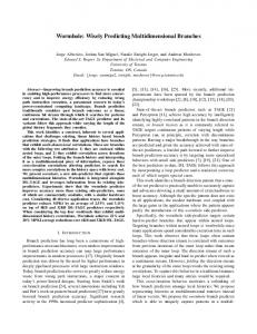
Figure 4. Gated Clock Error Library specification mismatches on the priority of clock and reset line contests may also cause the test model to behave erroneously when compared to its transistor level implementation. The other two categories include errors that relate to different multiplexer and multiplexer-latch implementations shown in Figure 3. In that figure, a triangle with no circle indicates a tristate buffer. It can be shown, with the use of appropriate truth tables [10], depending on the input values of each module, the output may be different. In practice, an extraction error arises from any replacement of one module for another. For example, one module implementation from the three implementation types shown in Figure 3(a) maybe mistakenly implemented with another module from Figure 3(a), etc. The net result is that this module misplacement may produce an erroneous test model that misleads test generation.

3 Error Types in Clocking Circuitry In this section we present a set of extraction error types that are common to the clocking circuitry of high-performance cores for microprocessors, SoCs, ASICs, etc in the industry today [2][3][5].

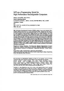
3.1 Gated Clock Modern devices impose strict power consumption and reliability requirements. Since not all design components may always need to operate simultaneously, the gated clock scheme of Figure 4(a) is commonly used to disable clocking of temporarily inactive components and save power [2][5]. The hardware in that figure is built in such a way so that the Local Clock 1 operates in the frequency of Global Clock 2 as long as Enable is at a logic 1.

Enable

Enable Global Clock

D Q

D Q

Local Global Clock1 Clock

(a)

Local Clock2

(b) Glb Clk Enable Loc Clk1 Loc Clk2

Stretch1 Stretch0

Adjustable Delay Buffer

Local Clock1

Enable1 Medium freq. pulse clk phase1

Enable2 Global Clock ClkBuf Type 1

(a)

(c) Figure 5. Frequency Divider Error Different implementations of the gated clock are shown in Figure 4(b) and 4(c). As seen, these implementation differ on the position (if any) of a NOT gate. An extraction process may erroneously replace one implementation with another during mapping for the flattened netlist. The waveforms for all implementations are found in Figure 4(d). We observe, that for the same input, they all produce different local clock results.

Stretch1 Stretch0 Enable1 Enable2 Global Clock

Stretch1 Stretch0 Enable1 Enable2 Gclk

Local Clock2 ClkBuf Type 1

Medium freq. pulse clk phase2

(b) Stretch1 Stretch0 Enable1 SlowClkSync Global Clock

Stretch1 Stretch0 Enable1 Enable2 Gclk

Local Clock3 Slow freq. ClkBuf Type 2 or 3 pulse clk phase1

(c) 3.2 Local Clock Frequency Divider Frequency dividers are used on approximate domain global clocks to generate integral local clock frequencies that drive various design blocks at different speed [3][5]. Figures 5(a) and 5(b) contain common hardware to implement such dividers. If the extraction process erroneously introduces a NOT gate at the input of the Enable line, the new local clock generated will be enabled at complementary phase (Figure 5(c)). This may result in a circuit malfunction because the memory elements of the core will lock/propagate different logic values.

Glb Clk Loc Clk1 Loc Clk2 Loc Clk3

(d) Figure 6. Clock Pulsed Buffer Error

3.3 Local Clock Pulsed Buffers

4 Debugging Pipelined Designs

Local clock buffers are used to generate clocks of a desired frequency for various design blocks [3][5]. These buffers are driven from global clocks through delay-matched taps. Different local clocks drive the various critical and non-critical units of the microprocessor in appropriate frequencies that guarantee performance yet save power. These buffers are available as pulsed and nonpulsed. Non-pulsed drivers simply buffer the input global clock and they usually present no problem to the extraction process. Figure 6(a) shows a medium pulsed clock driver. At the rise of the global clock, the pull-down path is asserted to generate the rising edge of the local clock. At the same time, the self-reset pullup path is asserted to generate the falling edge of the clock. The delay buffer is adjustable to permit different types of duty cycle for the output local clock. Variations of the hardware in Figure 6(a), shown as a box in Figure 6(c), allow for pulsed buffers that generate slow and fast frequency local clocks from global clocks. We omit these hardware descriptions that can be found in [5]. Additionally, Figure 6(b) shows the schematic for another medium pulsed clock driver with complementary phase to the one of Figure 6(a). During extraction, erroneous mapping or mismatches in library specifications may utilize a different pulsed buffer in place of the other. For example, a medium frequency buffer may be accidentally replaced with a slow frequency one or with one with inverted phase. From real life experience, it is usually unlikely that a fast frequency buffer will be replaced by a slower one, although the debugging method, presented next, can handle this case. When a pulsed buffer replacement error occurs, it may change the functionality of the test model and the input/output vectors collected in test generation may give faulty output responses during vector validation.

In this section we present an automated simulation-based debugging method for single extraction errors. Automated debugging involves two steps namely diagnosis and correction. Diagnosis identifies lines in the circuit where error effects may originate and correction proposes a module modification (replacement) on these lines to rectify the design. These modifications are selected from the types of extraction errors presented in the previous two sections. Since module mapping information is known to the engineer, it suffices for diagnosis to identify a single line driven by an error module. All other lines with similar erroneous modules are discovered by using the mapping information. One basic ingredient of diagnosis is a enhanced path-trace procedure. Path-trace is a line marking algorithm originally proposed by Venkataraman and Fuchs [9] to aid fault diagnosis. In the current work, we modify the procedure to accommodate the needs of the problem. The modified procedure simulates an input vector with failing responses and begins by marking an erroneous primary output. Subsequently, if the output of a gate is marked and all its inputs have non-controlling values, path-trace marks all inputs of the gate. If the output of a gate is marked and its inputs have one or more controlling values, path-trace randomly marks one such input. If the output of a gate is marked and its input have only logic unknown (X) and/or non-controlling values, path-trace marks all input that has an X. Finally, if the gate is a memory element, its input, reset and clock lines are always marked. Due to the pessimistic nature of path-trace, it can be shown that it always marks at least one line driven by an error module. We omit the proof of this claim which is similar to the one found in [7] that contains another 3-valued variation of path-trace.

Additional care needs to be taken once path-trace marks the output of some memory element of the pipeline. Although the procedure correctly marks (among other lines) the input of the flip-flop, the logic values in the circuitry of the fan-in cone of this input may be obsolete. This is because of the different clock domains that trigger independently and may change the values of the lines in the fan-in cone that feed the marked flip-flop. To elaborate further, consider the architecture in Figure 2 and assume that the memory elements in register files I and II are triggered by two independent clock domains as shown in Figure 7. Furthermore, assume that flip-flop F in file II driven by clock1 is marked by path-trace at time-frame t7 . In other words, path-trace started from an erroneous output marking lines in combinational circuitry C as it reaches the output of F . The reader may verify that any error effect that propagates to F , it did so using logic values in combinational circuitry B that corresponds to time frame t5 (or before), that is, prior to the trigger of clock1. This is because local clocks (including clock1) may be shared with register file I and overwrite the values in circuitry B past time frame t5 when clock1 triggers to store values in F. Since these values are now lost, we need to devise a way to restore them so that path-trace continues marking lines at the input of F correctly. Equivalently, if logic values in circuitry B are updated correctly and a memory element in register file I is marked, we need to restore all values of the gates in combinational logic A at time frame t3 to have path-trace continue marking lines correctly. The above discussion indicates that one needs to store the logic values of each logic primitive of the core for all time frames as different clocks trigger. These stored values can be recovered to guide path-trace to mark suitable sets of lines at appropriate time-frames. In the proposed implementation, these logic values are stored in the file registry and the primary input of the circuit. This is done with respective storage tables updated appropriately throughout the simulation of the circuit. Once an erroneous primary output is observed, the stored table values are simulated in the combinational block they fan out to restore the logic values on the primitives at correct time frames. We illustrate the need and utilization of the storage tables with an example.

0

1

1

1

D Q

IN0 Clock1

F1

0

D Q

Clock2

0

1

OUT0

0

X

X

X

X

X

X

D Q

IN3

X

OUT1

D Q

Clock1

X

1

F2

IN2 X

X

F4

Clock2

1

IN1

X D Q

F5

F3

Clock1

Error Module

(a) 1

0

D Q

IN0

0

0 D Q

F1 Clock1

Clock2

0 1

1

D Q

IN1 0

Clock2 0

0

Clock1

X

X OUT0

0

F2

IN2 0

X

F4

D Q

0

X

1

1

X

D Q

X OUT1

F5 F3

Clock1

IN3

(b)

PI Table I

PI Table II C1

C1 C2 IN0 0 IN1 0 IN2 0

0 0

IN3 1

1

0

C2

C1 C2 C1 C2 IN0 X X X X IN1 X X X X IN2 X X X X IN3 X X X X

PI Table I

PI Table II C1

C1 C2 IN0 1 IN1 1 IN2 0

0

IN3 0

1

0 0

C2

C1 C2 C1 C2 IN0 0 0 X X IN1 0 0 X X IN2 0 0 X X IN3 1 1 X X

RFI Table

RFI Table

C1 C2 F1 1 X F2 1 X F3 X X

C1 C2 F1 X X F2 X X F3 X X

(c)

(d)

Clock1

Figure 8. Error Circuit for Example 1 (a) first vector (b) second vector (c) storage tables at t1 (d) storage tables at t3

Clock2 t0

t1

t2

t3

t4

t5

t6

t7 t8

Figure 7. Example Clock Waveform Example: Consider the circuit in Figure 8(a) with Register Files RF I = {F1 , F2 , F3 ) and RF II = {F4 , F5 } and combinational core A, B and C that contains a single error with a single instantiation. This is the multiplexer implementation, shown within the dotted box, that needs be replaced with the leftmost (inverted) module from Figure 3(a). Assume the two clocks of the design have the timing characteristics from Figure 7. In the same figure, the aforementioned tables are also shown. Observe, a pair of tables is dedicated to the Primary Input (PI) and a single table to register file RF I. The column marked as C1 (C2) corresponds to information that pertain to Clock 1 (Clock 2). These tables do bookkeeping of logic values throughout simulation and they are updated at every clock trigger as follows. All entries of P I Table I are initialized to logic unknown X. Assume that at time t0 the first input vector 0001 is applied at the input. This vector excites the error and error values propagate to RF I. At time t1 , both clocks trigger and all the tables are updated as shown in Figure 8(a) to reflect logic values of the memory elements and the primary input prior to that clock trigger. The RF I table is updated first with the original values of the flip flops in RF I. In this case, all memory elements are initialized to X. Since both clocks trigger, all columns of the P I Table II are

overwritten by two copies of P I Table I. Intuitively, the first (last) two columns of Table II hold the value of the primary input prior to the last Clock 1 (Clock 2) trigger. Finally, both columns of P I Table I are updated with the input vector. After the tables are updated, the values are latched in RF I and simulated in the circuit for time-frame t1 . In that figure, the faulty values at the fan out cone of the error site are shown in circles. At time t2 , assume that the second input vector, 1100 is applied. At time t3 , only Clock 1 triggers and portions of all the tables are updated as shown in Figure 8(b). Since only Clock 1 triggers, only respective columns of the three tables are updated as explained earlier. These columns are shown in bold in that figure. Observe, column C1 of RF I table memorizes the logic values stored at the RF I flip flops at time frame t1 (circuitry in Figure 8(a)). It can be seen, after the tables are updated and the values are latched/simulated, error effects are observed at the primary output of the circuit. Once the errors are observed, path-trace is performed on combinational core C and it temporarily stops at F5 . Since this flip flop is controlled by Clock 1, the primitives in register file RF I are updated with the values in the C1 column of the RF I Table in Figure 8(b). Next, combination logic B is simulated to restore values and path-trace continues in B to stop at F3 . Since F3 is controlled by Clock 1, primary input values are restored from the (C1,C1)

Algorithm 1 Table Update and Enhanced Path-Trace 1: TP I 1 := PI Table I 2: TP I 2 := PI Table II 3: TRF := RF I Table 4: C := Clocks triggered at time t 5: RF I := the set of registers in Register File I 6: P I := the set of primary inputs 7: 8: 9: 10: 11: 12: 13: 14: 15: 16: 17: 18: 19:

procedure U PDATE TABLE(TP I 1, TP I 2, TRF , C, RF I, P I) for all c ∈ C do for all f ∈ RF I do TRF (c, f ) ← the state of f end for TP I 2(c) ← TP I 1 end for for all c ∈ C do for all i ∈ P I do TP I 1(c, i) ← the value of i end for end for end procedure

31:

procedure E NHANCED PATH TRACE(TP I 1, TP I 2, TRF , C, RF I, P I) path-trace on comb. circuitry C RF 2List ← marked registers in RF 2 for all r1 ∈ RF 2List do c1 ← clock of r1 read and place values in TRF (c1 ) on registers in RF 1 simulate and path-trace comb. circuitry B RF 1List ← marked registers in RF 1 for all r2 ∈ RF 1List do c2 ← clock of r2 read and place values in TP I 2(c1 , c2 ) on P Is simulate and path-trace on comb. circuitry A

32: 33: 34:

end for end for end procedure

20: 21: 22: 23: 24: 25: 26: 27: 28: 29: 30:

column of P I Table II. Once these input values are simulated in block A, path-trace continues to mark the error location.  Algorithm 1 contains pseudo code for the procedure U P DATE TABLE that updates the storage tables at every clock trigger during simulation. The same figure contains the pseudo code for E NHANCED PATH T RACE that uses these values to assist pathtrace in diagnosis. This is also the central procedure used in diagnosis. The first procedure works as follows. For every clock c ∈ C triggered at time t, the RF I Table is updated first with the current values of the flip-flops in register file I (line 10). Next, the PI Table II is updated by copying PI Table I to the column which is mainindexed with c (line 12). Intuitively, the columns of PI Table II under the same main index contain the values of the primary inputs prior to the last indexed clock triggered. Finally, the PI Table I is updated with the input vector (line 16). The values stored in the tables are used appropriately by E N HANCED PATH TRACE to restore logic values in the core circuitry and assist path-trace during diagnosis. When path-trace marks the registers in register file II, it reads the proper entry in RFI Table, and retrieves the correct values in combinational circuitry B by simulating the circuitry with the values read from the table. Then, pathtrace proceeds by marking in the combinational circuitry B (lines

24-26). When path-trace reaches the registers in register file I, it again reads the entry in PI Table II according to clocks controlling the registers on the path and restores the states of the lines in combinational circuitry A. Path-trace continues marking in core circuitry A and terminates when it reaches a primary input of the circuit, as explained earlier. These actions are taken in lines 29-31. After path-trace returns a set of candidate error locations, the algorithm ranks these locations in terms of path-trace counts and enters correction where error sites are visited in descending order of marks by path-trace. All potential error modifications are exhaustively enumerated on these sites and the circuit is re-simulated for the input test vectors. Corrections that return correct primary output results for the test vectors qualify debugging. For example, once diagnosis returns the error site pointed in Figure 8(a), correction will enumerate candidate correction models from Figures 3(a) and 3(c) to find that both modules qualify. ckt A B C D

primit. count 2197 3603 5034 7836

FF count 210 749 871 2876

ckt E F G H

prim. count 10046 13086 23978 36654

FF count 3787 3055 4663 8963

Table 1. Circuit Characteristics ckt

A B C D E F G H Avg

# of module Brute PathForce Trace 30.0 9.6 30.6 11.3 32.0 12.1 30.6 13.7 31.3 10.2 31.3 15.4 32.3 12.6 31.0 14.6 31.1 12.4

BruteForce 32.5 87.4 149.5 170.4 109.1 136.8 88.5 321.1

time (sec) Proposed One All 4.4 9.8 26.4 35.6 29.7 43.6 42.4 64.4 16.8 24.5 54.6 70.5 24.9 40.0 101.0 161.2

Speed up 3.3 2.5 3.4 2.6 4.5 1.9 2.2 2.0 2.8

Table 2. All State Equivalence Designs

5 Experiments Tests are carried on two-stage pipelined sequential designs (Figure 2) built with modified ISCAS’85 and ITC’99 combinational cirR cuitry on a Pentium 2.8 GHz processor. The clocking circuitry of these circuits consists of a scheme of 4 global clocks that drive 21 local clocks. The frequency of the global clock domains is an integral multiple of each other. The circuit names, primitive count and memory element count are found in Table 1. There is a total of 11 different types of extraction errors presented here and in [10]. To emulate a real physical synthesis environment, we realize 2-3 different module libraries for each error type for a maximum of 33 module types. In practice, this indicates a set of modules with the same functionality but different physical characteristics. For each circuit, we perform three types of experiments using the debugging algorithm from Setion 4 where all information, some (partial) information and no information of state equivalence is known, respectively. In the case of partial state equivalence, we randomly utilize 50% of the state equivalence information. Each experiment contains averages of 15 runs and times are in seconds. To exhibit the effectiveness of the proposed debugging approach, we compare its performance with a brute-force method where the engineer debugs the design manually by simply enumerating all module libraries. This brute-force approach is the common

A B C D E F G H Avg

# of module Brute PathForce Trace 30.0 24.7 30.6 17.2 32.0 19.9 30.6 23.6 31.3 21.3 31.3 29.6 32.3 30.9 31.0 29.6 31.1 24.6

BruteForce 47.7 134.9 228.9 259.1 170.2 233.3 178.9 566.6

time (sec) Proposed One All 10.8 21.5 22.3 61.5 43.5 108.3 78.7 142.3 20.3 61.6 115.4 215.9 74.1 106.4 124.4 369.9

150

Speed up 2.2 2.2 2.1 1.8 2.8 1.1 1.7 1.5 1.9

Table 3. No State Equivalence Designs ckt

A B C D E F G H Avg

# of module Brute PathForce Trace 30.0 5.9 30.6 10.8 32.0 11.9 30.6 12.3 31.3 8.3 31.3 14.3 32.3 11.7 31.0 12.8 31.1 11.0

BruteForce 51.4 132.5 226.5 256.3 170.0 601.6 247.6 486.8

time (sec) Proposed One All 3.8 8.9 26.4 50.1 60.0 90.5 62.7 99.9 25.7 38.7 65.3 88.6 29.2 48.1 120.9 185.0

120

Total CPU Time (sec)

ckt

Circuit A Circuit C Circuit D Circuit E

90

60

30

0

Full

Partial

None

Equivalence Information

Figure 9. Run-time vs. State Information Speed up 5.8 2.6 2.5 2.6 4.4 6.8 5.1 2.6 4.1

6 Conclusion This paper investigates discrepancies during extraction in test model generation of high-performance designs. Different classes of extraction errors in modern clocking schemes are presented. A diagnosis algorithm for single extraction errors in designs with no/partial state equivalence with the transistor level schematic is also proposed. Experiments demonstrate its efficiency that helps improve extraction and shorten the test delivery turnaround time for high-performance ICs.

Table 4. Partial Equivalence Designs

References debugging practice in the industry today when the test model fails since conventional design error techniques do not apply due to the different nature of the errors. Tables 2, 3 and 4 contain results for the all-, no- and partialstate equivalence case, respectively, presented in a similar manner as follows. The first column has the circuit name. Debugging results shown in the remaining columns are based on simulation of 2,000-3,000 erroneous vectors with high fault coverage (> 90%). The next two columns contain the average number of modules examined by manual debugging (brute-force) versus the one marked by path-trace. We observe, the enhanced path-trace has good resolution as it eliminates more than 40% (on the average) of useless module enumerations. The next three columns contain CPU times for the brute-force and the proposed debugging algorithm; Column 4 contains the time for the brute-force method to find all possible solutions, column 5 the respective time for the proposed approach to find one solution and column 6 the time to find all solutions. The solution may not be unique due to fault equivalence [8]. As seen from the speed up ratio (last column), the proposed approach reduces the effort dedicated to test model debugging by a factor of 3 when it searches for all solutions. The same experiments (not reported here) also show that the speed up is approximately 11 times when the method exits after the first solution. Figure 9 plots the run-times of the different cases of state equivalence information availability from Tables 2, 3 and 4 for four circuits. In three cases the CPU saving due to the information provided by the state equivalence is reflected in the final debugging effort. This is expected because state equivalence eases the task of path-trace as it reduces the number of time frames it has to traverse. In fact, this is the case for all circuits in our experimental set up except circuit A (dotted line) where the run time does not monotonically reduce as more state information becomes available. This is because the number of candidates marked by path-trace varies and it has an impact in the overall debugging time. In the future, we plan to investigate other discrepancies in test model generation for different circuit architecture types with feedback and further refine the debugging approach.

[1] M. Abadir, J. Ferguson, and T. Kirkland. Logic verification via test generation. IEEE Trans. CAD, 7:138–148, January 1988. [2] H. Ando, Y. Yoshida, A. Inoue, I. Sugiyamal, T. Asakawa, K. Morita, T. Muta, T. Motokurumada, S. Okada, H. Yamashita, Y. Satsukawa, A. Konmoto, R. Yamashita, and H. Sugiyama. A 1.3-ghz fifth-generation sparc64 micrprocessor. IEEE Journal of Solid-State Circuits, 38(11):1896–1905, 2003. [3] D. Bearden, D. Caffo, P. Anderson, P. Rossbach, N. Iyengar, T. Petrsen, and J.-T. Yen. A 780mhz powerpc microprocessor with integrated l2 cache. IEEE ISSCC, pages 90–91, 2000. [4] S. Kundu. GateMaker: A Transistor to Gate Level Model Extraction for Simulation, Automatic Test Pattern Generation and Verification. IEEE ITC, pages 372–381, 1998. [5] N. Kurd, J. Barkatullah, R. Dizon, and T. Fletcher. A multiR gigahert clocking scheme for the pentium 4 microprocessor. IEEE Journal of Solid-State Circuits, 36(11):1647–1653, Nov. 2001. [6] M. Kusko, B. Robbins, T. Snethen, P. Song, T. Foote, and W. Huott. Microprocessor test and test tool methodology for the 500mhz ibm s/390 g5 chip. Proc. IEEE ITC, 1998. [7] J. Liu, A. Veneris, and H. Takahashi. Incremental diagnosis of multiple open-interconnects. Proc. IEEE ITC, pages 1085– 1092, 2002. [8] A. Veneris and I. Hajj. Design error diagnosis and correction via test vector simulation. IEEE Trans. CAD, 18(12):1803– 1816, December 1999. [9] S. Venkataraman and W. Fuchs. A deductive technique for diagnosis of bridging faults. Proc. IEEE ICCAD, pages 562– 567, 1997. [10] Y. Yang, J. Liu, P. Thadikaran, and A. Veneris. Extraction error diagnosis and correction in high-performance designs. Proc. IEEE ITC, pages 423–430, 2003.