In this work, we propose to compute the Betti numbers from a generative model based on a simplicial complex learnt from the data. We compare it to the Witness ...
Extraction of Betti numbers based on a generative model Maxime Maillot12 , Micha¨el Aupetit1 and Gerard Govaert2 1- CEA, LIST, Information, Models and Machine Learning Laboratory (LIMA) F-91191 Gif-sur-Yvette, France 2- University of Technology of Compiegne - Heudiasyc BP 20529 F 60205 Compi`egne, France Abstract. Analysis of multidimensional data is challenging. Topological invariants can be used to summarize essential features of such data sets. In this work, we propose to compute the Betti numbers from a generative model based on a simplicial complex learnt from the data. We compare it to the Witness Complex, a geometric technique based on nearest neighbors. Our results on different data distributions with known topology show that Betti numbers are well recovered with our method.
1
Introduction
Exponential growth of sensors and databases leads to more and more multidimensional data to process. The analyst needs new exploration tools to get more relevant summaries of these data. Unsupervised learning methods usually extract some relevant variables or combinations of variables using dimension reduction techniques, or summarize the data instances straight into the multidimensional space using clustering techniques [1]. Here we focus on a topological summary of the data. Interesting topological invariants are preserved through homotopy, a very large class of nonlinear transformations which includes homeomorphism, similarities and isometries as nested cases. Thus these invariants are more robust than geometrical or statistical properties. So they are more likely to survive the processing chain from the set of sensors observing the physical phenomenon under study, to the set of instances and variables finally used to describe this phenomenon. In this work, we focus on the extraction of such topological invariants from the data set.
2
State of the art
We assume that data are drawn from a set of manifolds in RD (the population) following some probability density function (pdf) corrupted with noise. Gaussian Mixture Models (GMM)[1] are generative models which attempt to estimate the population pdf from the data sample with a linear combination of Gaussian pdf. The GMM can also be used for a clustering purpose, where each component accounts for some part of the population. This latter point of view assumes that the population is a set of generative points (the mean vector of each Gaussian component), i.e. 0-dimensional manifolds corrupted with Gaussian noise (the Gaussian pdf of each component). From a topological point of view, this
model is very simple as it encodes the data as a set of disjoint point-sources. Some attempts have been made to extract more topological information from the data. Generative models in the spirit of Self-Organizing Maps [2], like the Generative Principal Manifolds [3] or the Generative Topographic Maps [4] have been proposed but they impose a priori the manifolds to be connected and one or two dimensional. In our previous work [5, 6], we proposed the Generative Gaussian Graph similar to the Topology Representing Network [7], to learn the connectedness of the population in a statistical learning framework. We defined a weighted Delaunay subgraph of some prototypes located with a GMM, and use convolution of this graph with a Gaussian pdf as the basis of a generative mixture model. Vertices and edges of the graph are the components of the mixture. Proportions of the components are tuned to maximize the likelihood. Edges with low proportions are pruned from the graph so that remain only edges and vertices which explain the data. In the field of Computational Topology, new tools have been proposed to extract more subtle topological information from the data than the connectedness. The Betti numbers are such information which count the number of unconnected component in each dimension. For instance, a sphere has one connected component, no hole and one cavity, its Betti numbers are (1,0,1,0,0,...). More details about these topological notions can be found in [8]. Betti numbers provide a topological signature of manifolds which allows to classify them according to some characteristics of their topology. The basis to compute Betti numbers is to model the data with a simplicial complex. A simplical complex C is a collection of simplices S such that for any two simplices Si and Sj in C, their intersection is either empty or in C. A k-simplex is a set of (k + 1)-vertices which can be embedded in RD≥k as the convex hull of k + 1 points in independent position : a 0-simplex is a point; a 1-simplex is a line segment; a 2-simplex is a triangle with its interior; a 3-simplex is a tetrahedron with its interior... The Witness Complex (WitC) have been proposed in [DeSilva04]. It extends the Topology Representing Network (TRN) from Delaunay subgraphs to Delaunay simplicial complexes. In WitC, a set of vertices (0-simplex) is defined subsampling the data or using some vector quantization technique. For each data, the two nearest vertices to it are connected with an edge (1-simplex). A data which leads to the creation of a simplex is called its ”witness”. At that point, the algorithm is identical to the TRN. Then for each data, the three nearest vertices to it define a triangle (a 2-simplex) except if one of its edges (1-face of the 2-simplex) has no witness. And so on, for each data, the k nearest vertices to it define a (k−1)-simplex of the Witness Complex except if one of its (k−2)-faces has no witness. The obtained Witness Complex is a simplicial complex whose topology is intended to catch the one of the population underlying the data. This technique is essentially a geometrical one and it has some limits among which : it is sensitive to noise; no statistical criterion is optimized; the witness complex is not self-consistent as points densely drawn from its embedding may not give rise to it although based on the very same set of vertices. In the sequel, we propose to extend the Generative Gaussian Graph to a
generative simplicial complex model and we compare it to the Witness Complex while extracting Betti numbers from some sampled manifolds.
3
The Generative Simplicial Complex
In this paper, we assume that the data are vectors of RD drawn from a collection of manifolds corrupted with a centered gaussian noise, whose variance σ 2 is unknown. We assume that this collection of manifolds can be approximated with a Delaunay simplicial complex of some vertices located in RD . We define the Generative Simplicial Complex (GSC) as such a model, and use the EM method [9] to tune its parameters and maximize its likelihood. 3.1
The generative simplex
A gaussian simplex is the elementary component of the Generative Simplicial Complex. It is a probability density function. Let S d be a simplex of dimension d with d + 1 vertices in RD , |S d | its volume,g a D-dimension gaussian distribution, σ > 0 the standard deviation, and p the propability distribution induced by the gaussian simplex associated with S d . Then Z ||(x−t)||2 1 1 − 21 d 2 σ2 g(x|v, σ 2 )dv with g(x|t, σ 2 ) = e p(x|S , σ ) = |S| S d 2π D/2 σ D We use a quasi Monte-Carlo method to evaluate this multi-dimensional integral [10]. 3.2
From the Generative Simplex to the GSC
A Generative Simplicial Complex is a mixture of generative simplices. Let Sid be the i-th simplex of dimension d, πid its weight in the mixture model, p(x|Sid , σ 2 ) its probability density function, D the maximum dimension of a simplex in the model, nd the number of simplices of dimension d, σ the standard deviation (the same for every simplex), and Dt ≤ D the current dimension in the iterative algorithm. Then : p(x|t) =
nd Dt X X
πid p(x|Sid , σ 2 )
d=0 i=1
4
The learning process
Given a data set, a generative simplicial complex can be learnt from this data, to approximate the underlying manifold.
4.1
Initialization
This step gives us a set of prototypes in RD that we will use as the vertices of the GSC. We use a classical Gaussian Mixture Model where the prototypes will be the center of the gaussian distributions optimized thanks to the ExpectationMaximization [9] algorithm. The selection of the number of prototypes is made using the BIC criterion [11]. 4.2
Building the initial complex
We build the Delaunay simplicial complex in dimension D with the prototypes. We sort the simplices by increasing dimension. These simplices are the components of the GSC model. In the next step we want to prune this GSC, to get another one that would better fit the data with respect to the likelihood. 4.3
Iterative building of the GSC
We start with the vertices and the edges belonging to the GSC, we have a partial GSC of dimension 1 (Dt = 1). Step-by-step, we will add the triangles (Dt = 2), then the tetrahedra (Dt = 3) and so on until Dt = D. At step t, we have a Dt -dimensional GGSC. During each step, we maximize the likelihood, using EM, only to optimize the weights π. They are initialized as : 1 πid = PDt
j=0
nj
After convergence, if a weight πid is below a certain threshold s, the simplex is automatically removed from the GGSC ie πid = 0. If a simplex has a weight πid ≥ s, its facets of lower dimension are removed from the GGSC. Sid
4.4
Getting the Betti numbers
Now that we have a pruned GSC, we use Plex [12] to get its Betti numbers.
5 5.1
Experimentations Checking the validity of the model
These first experiments shows that learning with a GSC is possible on elementary simplices. It also gives us a threshold to prune the GSC after each step described at 3.3. The data are generated using a GSC model. A simplex of dimension d will compete with simplices of dimension d − 1. We want to be sure that the model can learn the intrinsic dimension of the data, which is among the basic topological information we want to learn. For example, three segments forming a triangle are competing with the interior of the triangle and vice-versa. We set the vertices of the GSC on the ones used to generate the data, and set the noise to σ = 0.05, in the data and in the model. We also set the threshold at a tenth of the initial weight values.
In each case, the algorithm is capable of making a distinction between a simplex of dimension d and its hull of intrisec dimension d − 1. 5.2
Learning the Betti numbers on a random simplicial complex
We generate data from a random simplicial complex, drawn from the elementary simplex of dimension 5, with a noise σ = 0.05. We get non trivial topology with such a complex. We set the vertices of the GGSC on the ones used to generate the data. The algorithm is capable of dealing with different intrinsic dimensions. We only compare the Betti numbers of the generated random complex to the ones learnt from the GGSC. The following table gives the results. It is possible to learn the Betti numbers from data generated by a simplicial complex.
GGSC
σ = 0.005 87.00%
σ = 0.01 83.00%
σ = 0.05 95.00%
Fig. 1: Betti numbers learning with different noises
5.3
Learning the Betti numbers of a sphere and a ball
Two data set will be used in this experiment : a sphere, of radius one corrupted with three different noise variances, and a ball of the same radius, also corrupted with the same noise. Betti numbers of the sphere are (1,0,1,0,...), Betti numbers of the ball are (1,0,0,0,...). Data are generated in a three dimension space. 30 vertices will be used for the learning (30 was the number given after running the GMM with BIC on the data).
σ = 0.005 σ = 0.01 σ = 0.05
WitC 0.00% 0.00% 1.00%
GGSC 0.005 83.00% 90.00% 95.00%
GGSC 0.01 0.00% 98.00% 89.00%
GGSC 0.05 0.00% 0.00% 87.00%
Fig. 2: Succes rate of extracting Betti numbers of a sphere made of 2000 points corrupted with noise σ
σ = 0.005 σ = 0.01 σ = 0.05
WitC 50.00% 56.00% 1.00%
GGSC 0.005 100.00% 89.00% 0.00%
GGSC 0.01 86.00% 97.00% 0.00%
GGSC 0.05 0.00% 0.00% 87.00%
Fig. 3: Succes rate of extracting Betti numbers of a ball made of 4000 points corrupted with noise σ The model can have good performance, but it really depends on the variance parameter. Such a parameter does not exist in WitC. WitC results on the sphere
Fig. 4: Data used for learning the Betti numbers of a sphere
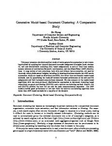
Fig. 5: Generative model learnt from a distribution of a sphere
can be explained by its weakness towards noise. The sphere problem is the most difficult because a 2-dimension manifold is corrupted by a 3-dimension noise.
6
Conclusion
The GGSC is the first generative model capable of extracting the Betti numbers of data drawn from a manifold, corrupted with noise. If the second Betti number or upper is non-zero, it means there are cycles or holes in the data : projection in lower dimension may contain tears or false-neighbourhood. It has a dependancy on the variance parameter, that we will try to learn automatically in the future. It takes about three minutes to compute a GGSC in the case of the sphere; computing the initial probabilities and the Delaunay Complex are the two longest steps. We compared the algorithm to the geometrical part of WitC, but we should compute in the future the persistance of homology to be more accurate.
References [1] Geoffrey McLachlan and David Peel. Finite mixture models. 2000. [2] T Kohonen. Self-organization and associative memory formation. 1988. [3] R Tibshirani. Principal curves revisited. In Springer, editor, Statistics and Computing vol. 2, pages 183–190, 1992. [4] Christopher Bishop, Markus Svens´ en, and Christopher Williams. The generative topographic mapping. In Neural Computation, pages 215–234, 1998. [5] Micha¨ el Aupetit. Learning topology with the generative gaussian graph and the em algorithm. In MIT Press, editor, Advances in Neural Information Processing Systems, pages 83–90, 2006. [6] Pierre Gaillard, Micha¨ el Aupetit, and G´ erard Govaert. Learning topology of a labeled data set with the supervised generative gaussian graph. In Neurocomputing, pages 1283– 1299, 2008. [7] Thomas Martinetz and Klaus Schulten. Topology representing networks. In Elsevier London, editor, Neural Networks vol. 7, pages 507–522, 1994. [8] Gunnar Carlsson. Topology and data. pages 255–308, 2009. [9] A Dempster, N Laird, and D Rubin. Maximum likelihood from incomplete data via the em algorithm. In Journal of the Royal Statistical Society, Series B, vol. 39, pages 1–38, 1977.
[10] W Morokoff and R Caflisch. Quasi-monte carlo integration. In Journal of Computational Physics, pages 218–230, 1995. [11] Gideon Schwarz. Estimating the dimension of a model. In The Annals of Statistics vol. 6, pages 461–464, 1978. [12] Vin de Silva. Plex - a matlab library for studying simplicial homology.