extraction of built-up areas using convolutional neural networks and

The International Archives of the Photogrammetry, Remote Sensing and Spatial Information Sciences, Volume XLII-3, 2018 ISPRS TC III Mid-term Symposium “Developments, Technologies and Applications in Remote Sensing”, 7–10 May, Beijing, China

EXTRACTION OF BUILT-UP AREAS USING CONVOLUTIONAL NEURAL NETWORKS AND TRANSFER LEARNING FROM SENTINEL-2 SATELLITE IMAGES V. S. Bramhe1,*, S. K. Ghosh 1, P. K. Garg1 1Geomatics

Engineering Group, Civil Engineering Department, IIT Roorkee, 247667,India, [email protected] Commission III, WG III/1

KEY WORDS: Built-up Area Extraction, Convolutional Neural Networks, Deep Learning, Sentinel-2 Images, Transfer Learning

ABSTRACT: With rapid globalization, the extent of built-up areas is continuously increasing. Extraction of features for classifying built-up areas that are more robust and abstract is a leading research topic from past many years. Although, various studies have been carried out where spatial information along with spectral features has been utilized to enhance the accuracy of classification. Still, these feature extraction techniques require a large number of user-specific parameters and generally application specific. On the other hand, recently introduced Deep Learning (DL) techniques requires less number of parameters to represent more abstract aspects of the data without any manual effort. Since, it is difficult to acquire high-resolution datasets for applications that require large scale monitoring of areas. Therefore, in this study Sentinel-2 image has been used for built-up areas extraction. In this work, pre-trained Convolutional Neural Networks (ConvNets) i.e. Inception v3 and VGGNet are employed for transfer learning. Since these networks are trained on generic images of ImageNet dataset which are having very different characteristics from satellite images. Therefore, weights of networks are fine-tuned using data derived from Sentinel-2 images. To compare the accuracies with existing shallow networks, two state of art classifiers i.e. Gaussian Support Vector Machine (SVM) and Back-Propagation Neural Network (BP-NN) are also implemented. Both SVM and BP-NN gives 84.31% and 82.86% overall accuracies respectively. Inception-v3 and VGGNet gives 89.43% of overall accuracy using fine-tuned VGGNet and 92.10% when using Inception-v3. The results indicate high accuracy of proposed fine-tuned ConvNets on a 4-channel Sentinel-2 dataset for built-up area extraction.

1. INTRODUCTION With the recent advancement in sensor technology, a large number of Remote Sensing (RS) satellites (Landsat, Sentinel, Worldview etc.) are available at different spatial resolution, fast revisit time as well as a wide variety of spectral bands. However, retrieving accurate information from remote sensing data is still a challenging task (Mukherjee, 2012).Satellite images have complex patterns that are difficult to understand due to its heterogeneity (Ashish, 2009; Adam, 2014). Identification of built-up areas is essential for territorial planning, climate change studies, population relocation etc. Since spectral features are not sufficient to extract built-up areas as other classes such as River Sand and Fallow Land shows similar spectral characteristics. Therefore, there is a need to develop more sophisticated algorithms in order to extract built up with precision using remotely sensed data. In present day context, traditional classifiers such as Support Vector Machines (SVM), Multi-Linear Perceptron (MLP), and Linear Regression (LR) are shallow structures. These networks process input data in single layer whereas, when using kernel function, the same input data can be processed in two layers (Melgani, 2004; Ustuner, 2015). Detecting urban areas in satellite images using traditional approaches requires human expertise and it is time consuming also. Most of the previous studies mainly focuses on classifying pixels or group of pixels by extracting low-level image features such as texture (Zhao, 2007), spatial and spectral information (Bernabe, 2014; Tuia, 2014) or hybrids (Tuia, 2009; Zhang, 2014; Tong, 2014). Spectral-spatial classification approaches are widely used in recent years for satellite image classification. The classification

algorithm improves the accuracy of classification by inclusion of spatial information (Benediktsson, 2003; Zhang, 2013). Spatial features such as Gray Level Co-occurrence (GLCM) derived texture features, Wavelets, Morphological Profiles etc. are widely used for urban area classification (Kuffe, 2016; Vu, 2003) Although satellite imagery provides continuous availability of data, it is a big challenge to accurately retrieve the extent of urban area using that data (Sirmacek, 2010). In Zhong (2007) various features are classified separately using Conditional Random Field (CRF) classifier and then information is fused to get the class information. The approach gives good accuracy but suffers from taking higher computational times because of multiple classifiers. In Sirmacek (2011) various local features are detected and used in detection of urban area using variable kernel based density estimation method. Gamba (2007) utilize the boundary information for urban area mapping. The boundary and non-boundary pixels are classified using neural network and Markov Random Field (MRF) classifiers respectively and the results are combined using decision fusion. They have come to get good mapping of VHR imagery. Performance of classifiers are highly dependent on representation of data or features. Erroneous or incomplete features limit the performance of classification; therefore, feature extraction is a key step that generally requires human intelligence and prior knowledge of the field (Arel, 2010). However, a Deep Learning (DL) algorithm is able to provide multiple higher level features, automatically without any feature engineering (Bengio, 2013). Deep learning approaches are giving impressive results in the field of pattern recognition. Recent studies suggested great potential of these methods in remote sensing also.

This contribution has been peer-reviewed. https://doi.org/10.5194/isprs-archives-XLII-3-79-2018 | © Authors 2018. CC BY 4.0 License.

79

The International Archives of the Photogrammetry, Remote Sensing and Spatial Information Sciences, Volume XLII-3, 2018 ISPRS TC III Mid-term Symposium “Developments, Technologies and Applications in Remote Sensing”, 7–10 May, Beijing, China

DL classifiers are well known to computer vision community still limited research has been carried out for RS data (Romero, 2016). However, in recent years, a shift towards the usage of DL techniques for various applications such as PAN sharpening (Masi, 2016), object detection, Land cover classification (Basu, 2015). Most of the studies using DL approaches have been carried out either on Aerial images or Very High Resolution (VHR) images such as UC Merced dataset or ISPRS Vaihingen and Potsdam benchmark data sets for image classification or semantic labelling.

nonlinear function. These models combine non-linear modules such that the data is being transformed to different representation and becomes more and more abstract after each level of processing. Deep Neural Network (DNN) models capture multiple representations, using hierarchical processing of data. These models process the input data sequentially in each module such that the output of the previous module is used as input to the next modules, these modules are called layers. Input and output units are connected through weights and biases whose values are learned during training of the network.

The primary objective of this paper is to test the suitability of pre-trained Convolutional Neural Networks (ConvNets) on Sentinel-2 images for built-up classification. Our goal is to develop an approach which can exploit DL technique specifically ConvNet to extract informative features that can accurately distinguish built-up areas in the Sentinel-2 images.

3. STUDY AREA AND DATA USED

2. HISTORY AND BACKGROUND The main goal of DL research is to solve our day-to-day tasks, which are highly complex for machines like recognising objects, Natural language processing (NLP) etc. Our brain can model the same physical world it sees regularly, so it can easily able to specify good priors for modelling the world. During 1960s, Hubel and Wiesel’s early work (Hubel, 1962; Hubel, 1965) on the cat’s visual cortex shows that visual cortex contains an intricate ordering of cells. These cells are sensitive to small context of the visual field, called a receptive field. Primary visual cortex is around seven stage beyond the retina. So, the information reaching visual cortex processed through multiple times, where at each stage higher level features are generated. Fukushima (1980), first discuss the concept of deep convolutional network. This network is similar to the structure of a human visual processing as discussed by Hubel and Wiesel’s work The output of this network was able to provide features that were not affected by position, change in shape and stimulus pattern. During 1970s and 1980s use of backpropagation to compute the gradient of objective function evolved significantly. The first practical demonstration of BackPropagation (BP) at Bell Labs was done by LeCun (1990). In this study, convolutional networks were trained using BP algorithm to classify handwritten digits. Auto encoders were also introduced during the late 80’s (Rumelhart, 1986; Baldi, 1989) as a technique for dimensionality reduction but these techniques are limited to compress the features in lower dimensions only. In 2006, a major breakthrough was achieved by unsupervised pre-training of Restricted Boltzmann Machines (RBMs) on MNIST data set (Hinton, 2006). An effective way of training deep networks has been presented in this study. Also, the work done by Bengio (2007) and Ranzato (2007) revived the interest of Machine Learning (ML) community in feed forward networks again. As one can see that the idea of multiple level processing of data has been formalized long before, but the main reasons behind success and widespread use are, the availability of high-end Graphical Processing Units (GPUs) and a large amount of labelled data available for training these days. Representation learning is a set of methods that allow a machine to be fed with raw data and to automatically discover the representations needed for detection or classification. (Hinton, 2007; Bengio, 2013). Better feature representation of data leads to good performance of classification. DL networks can model complex relationship between variables using multiple layers of

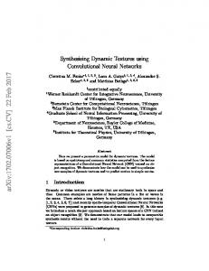
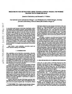
The study area selected comprises of Haridwar Tehsil, India. The coordinates of the bounding box covering study area is, Long. 77° 51' 21.00'' E and Lat. 30° 07' 0.31'' N at upper left and Long. 78° 20' 39.91'' E and Lat. 29° 38' 13.10'' N at lower right. Haridwar Tehsil is situated on the plane of the Ganges river.In last few decades, rapid urbanization has been taken place in this area, which results in increased infrastructural/ housing construction and urban expansion. The area comprises of heterogeneous land cover types including built-up regions, agricultural area, water, river sand and fallow land. The false colour composite image of the study area is shown in Figure 1.

Figure 1. False color composite (FCC) of Sentinel-2 (Band 8 (NIR), 4 (Red), 3 (Green)) of study area. The satellite data used in this study consists of fourmultispectral bands i.e. NIR, Red, Green and Blue acquired by Sentinel-2 Multispectral Imager (MSI) on 11 November 2016.The image represents a diverse land class scenario with pixels in four bands ranging from wavelength 0.49-0.842 µm in the electromagnetic spectrum. 4. METHODOLOGY In this section, various techniques used in this experiment along with proposed classification framework for built-up area extraction is discussed. 4.1 CNN Architecture CNN is one of the most popular computer vision algorithm today, due to its ability to handle image data effectively. As CNN model consists of multiple convolution and pooling operations therefore, it is very good at finding more abstract and robust representation of image features in the input data (Maggiori, 2017). In the case of CNNs, weights are shared

This contribution has been peer-reviewed. https://doi.org/10.5194/isprs-archives-XLII-3-79-2018 | © Authors 2018. CC BY 4.0 License.

80

The International Archives of the Photogrammetry, Remote Sensing and Spatial Information Sciences, Volume XLII-3, 2018 ISPRS TC III Mid-term Symposium “Developments, Technologies and Applications in Remote Sensing”, 7–10 May, Beijing, China

locally and weights connected to the same output unit form a filter (Romero, 2016). A CNN architecture consists of multiple convolution and pooling layers. To generate convoluted feature maps, kernel functions as filters are used in convolutional layers.The convoluted features are generalised into higher levels by subsampling layer which make features more abstract and robust. Similar to the structure in the primary visual cortex system where simple and complex cells are stacked layer-wise, convolution and pooling layers are intermixed in CNNs. The number of convolution and pooling layer can be different and generally depends on the application. To draw mathematical formulation, suppose we have a ddimensional input data x d , in case of multiband data, m is width, n is height and c is number of channels in input data x. Therefore, for a given input x, the output of any convolution layer lcan be defined as

N  hlj  f   hil 1  kijl  blj   i 1 

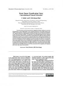
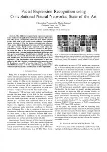
weight according to the application. In Penatti (2015) CaffeNet and Overfeat ConvNets are fine-tuned on remote sensing dataset for classification purpose. Experiment on these datasets suggests that Transfer Learning can be adopted for classifying satellite images also. Szegedy (2015) first proposed Inception (GoogleNet) architecture. This architecture won ImageNet competition. Since then the model is utilized in various computer vision applications because of its good performance and low computational cost in comparison to AlexNet or other architectures. In Castelluccio (2015) GoogleNet along withCaffeNet are trained to classify UC-Merced dataset and Braizilian Coffee Scenes.Inception-v3 uses 12 times fewer parameters than the winning architecture of AlexNet (Krizhevsky, 2012). In Figure 2. single module of Inception is shown.

(1)

where, f    is an activation function which could be sigmoid (Russell, 2003) , Rectified Linear Unit (ReLU) (Krizhevsky, 2012) or hyperbolic tangent . The  denotes convolution l

operation and N denotes number of input feature maps. kij is the kernel operating on ith feature map of layer l-1 to give jth feature l

map of layer l and b j is the bias for jth feature map of layer l. If l 1

l =1 then h  x is the input layer.Features generated by convolution layers are then given as input to pooling layer. Popular pooling functions are average pooling or sub-sampling and max-pooling (Lee, 2015). The output of sub-sampling can be defined as

S lj  g   lj   N N

 hlj1 

nn

b

l j

  

(2)

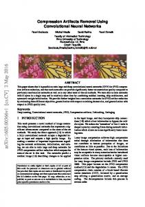
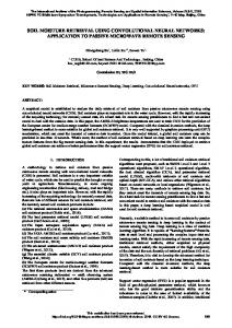
Figure 2. Inception module with dimension reductions (Szegedy, 2015) VGGNet was proposed by Simonyan (2014). This network adopts very simple design where only 3x3 convolution filters and 2x2 pooling layers are used. The size of input layer is 224x224, and then series of convolution and pooling layers are interspersed along with three fully connected layers and soft max classifier. The configuration of VGGNet is shown in Figure 3 (Simonyan, 2014)

where, the average of n  n patch of previous layer’s jth feature l 1

map i.e. h j is taken. Then, it is multiplied by a trainable scalar γ and adds to a bias b and passes through a non-linear function g    . Whereas, a max-pooling operation can be defined as (Scherer, 2010)

 

nn   l Q  max  hlj1  j N N  

(3)

In general pooling layers are inserted after convolution layers so that the spatial size and computational complexity would be reduced. Also, the features become more robust so the model will be less likely to over-fit. A very important feature of CNN is weight sharing in the convolution layers, so that same filter bank can be used for all pixels in a particular layer. 4.2 Inception-v3 and VGGNet A large amount of labelled dataset is a pre-requisite for success of any CNN. However, it is very difficult to collect large amount ground truth data in remote sensing studies. Therefore, it is easier to adopt an already trained network and update its

Figure 3. VGG Network Architecture proposed by Simonyan, (2014)

This contribution has been peer-reviewed. https://doi.org/10.5194/isprs-archives-XLII-3-79-2018 | © Authors 2018. CC BY 4.0 License.

81

The International Archives of the Photogrammetry, Remote Sensing and Spatial Information Sciences, Volume XLII-3, 2018 ISPRS TC III Mid-term Symposium “Developments, Technologies and Applications in Remote Sensing”, 7–10 May, Beijing, China

Both Inception-v3 and VGGNet models learn to explain better feature representation for different class of images. To train these models ImageNet Large-Scale Visual Recognition Challenge (ILSVRC) dataset is used. These models are initially trained on millions of images of generic objects such as table, pen etc. and able to categories them into 1000 object classes. 4.3 Classification Framework Following steps has been taken to classify built-up areas in order to implement transfer learning based approach: i. Download pre-trained Inception-v3 and VGGNet network ii. Patches centered over ground truth pixel location are extracted from Sentinel-2 image which are of same size of input layer of the networks. iii. Fine tuning of the networks on training dataset iv. Applied fine-tuned network on test dataset

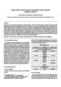
will be more scattered and randomly distributed all over the study area. To capture the spatial information contained within image, a local neighborhood of fixed size (patch)has been considered. The label of center pixel is taken as reference of output class. Image patches of fixed size around the center pixel of known class locations have been taken to train the network. Patch size taken from Sentinel-2 is taken as 11x11 because to capture small contextual variation present in the kernel. Figure 4 shows the sample patches used in training and testing of classifiers. However larger kernel size can also be taken but in that case pixels for different classes makes kernel less homogeneous and also causes smoothing effect on the output result (in case of generation of classified map). 16000 image patches centered over the known class location of built-up classes and other classes such as vegetation, water etc. have been extracted. Whereas, the accuracy has been tested over 4000 image patches. 5.2 Training and Validation

Firstly pre-trained networks with learning weights on ImageNet dataset are download. In order to employ these networks on new dataset final layers of the networks are replaced with fullyconnected, softmax and classification layer. Extraction of patches have been done which are centered over the known ground truth pixel. Once labelled data is generated fine-tuning of networks have been done. Finally, trained networks are applied on test dataset and accuracy of the networks are calculated. 5. EXPERIMENT AND ANALYSIS 5.1 Generation of Training and testing dataset The major problem when using CNNs for remote sensing studies is the availability of labelled data for training the network(Castelluccio, 2015). Since, collecting ground truth data is one of the difficult task some freely available datasets provided by various agencies and research groups are easier choice for training and testing of algorithm. Most commonly used dataset are hyperspectral scenes of Pavia and Salinas data. UC-Merced dataset consists of 100 samples of size 256x256 belongs to 21 classes which are extracted United States Geological Survey (USGS) National Map. AID dataset, having 30 different classes and about 200 to 400 samples of size 600x600 in each class. SAT-4 and SAT-6 datasets consists of 500000 samples of size 28x28 for 4 different classes.

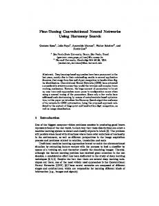
In this work, pre-trained ConvNets i.e. Inception v3 and VGGNetare used for transfer learning. Both of these networks are trained on ImageNet dataset, which consists of generic images of objects such as trees, vehicles, persons etc. Since, these networks are learned on ImageNet dataset, which are having very different characteristics from satellite images therefore, final layers of these networks are fine-tuned using data derived from Sentinel-2 images. To fine-tune the networks size of training images should be equal to the input size of the network, therefore, pre-processing (resizing, rotation and reflection) of data has been done. Figure 5 shows change in training and validation accuracy of the network at each iteration of VGGNet architecture.

Figure 5. Accuracy plot at each iteration of VGGNet training. The training run through 6 epocs (using all training data in the network) with 700 iterations in each. 70% of data is used for training whereas 30% is used for validating the model. It can be seen that both training and validation accuracy greatly increases initially but later there is very subtle increase at each iteration. In Figure 6 depicts cross-entropy error at each iteration of training and validation of VGGNet is shown. It can be seen that error of training data keeps on fluctuating whereas validation data error (shown by black dots) keeps on decreasing. Figure 4. Built-up area patches generated from Sentinel-2 dataset for training and testing networks For this study, training and testing samples have been taken using stratified random sampling method so that the samples

This contribution has been peer-reviewed. https://doi.org/10.5194/isprs-archives-XLII-3-79-2018 | © Authors 2018. CC BY 4.0 License.

82

The International Archives of the Photogrammetry, Remote Sensing and Spatial Information Sciences, Volume XLII-3, 2018 ISPRS TC III Mid-term Symposium “Developments, Technologies and Applications in Remote Sensing”, 7–10 May, Beijing, China

Ashish, D., McClendon, R.W., Hoogenboom, G., 2009. Landuse classification of multispectral aerial images using artificial neural networks. International Journal of Remote Sensing, 30(8), pp. 1989–2004. Baldi, P., Hornik, K., 1989. Neural Networks and Principal Component Analysis: Learning from Examples Without Local Minima. Neural Netw., 2(1), pp. 53–58.

Figure 6. Accuracy plot at each iteration of VGGNet training. 5.3 Accuracy assessment To compare the results of Inception-v3 and VGGNet two shallow network models i.e. Gaussian SVM (RBF-SVM) and Back-propagation Neural Network (BP-NN) are also tested on similar dataset. These classifiers have been chosen because they are most widely used classifiers in remote sensing classification. Out of the all, the labelled data 4000 patches have been kept for calculating the test accuracy. Table 1 shows the overall accuracy of classification of fine-tuned ConvNets in comparison to other shallow classifiers. Method

Classification accuracy (%)

BP-NN

82.86

RBF - SVM

84.31

Inception-v3

92.10

VGGNet

89.43

Table 1. Comparison of overall accuracies of Deep and shallow networks 6. CONCLUSIONS In this work, Transfer learning approach for built-up area classification is proposed. Experiments are carried out on Sentinel-2 image having four spectral band with 10 m spatial resolution. Weights of Inception-v3 and VGGNet models are fine-tuned with 16000 image patches. Whereas, 4000 image patches test are used to test the model. Results shows that Inception-v3 and VGGNet gives overall accuracies of 92.10% and 89.93% respectively, which is good improvement in comparison to BP-NN and RBF-SVM methods.Whereas, in between applied CNNs,the Inception-v3 model are faster to train in comparison to VGGNet due to their network structure. For future studies, effect of different kernel size on efficiency and generation of map of whole image will be considered.

Basu, S., Ganguly, S., Mukhopadhyay, S., DiBiano, R., Karki, M., Nemani, R., 2015. DeepSat. In Proceedings of the 23rd SIGSPATIAL International Conference on Advances in Geographic Information Systems - GIS ’15. New York, New York, USA: ACM Press, pp. 1–10. Benediktsson, J.A., Pesaresi, M., Arnason, K., 2003. Classification and feature extraction for remote sensing images from urban areas based on morphological transformations. IEEE Transactions on Geoscience and Remote Sensing, 41(9), pp. 1940–1949. Bengio, Y., Lamblin, P., Popovici, D., Larochelle, H., 2007. Greedy Layer-Wise Training of Deep Networks. Advances in Neural Information Processing Systems, pp. 153-160. Bengio, Y., Courville, A., Vincent, P., 2013. Representation Learning: A Review and New Perspectives. Pattern Analysis and Machine Intelligence, IEEE Transactions on, 35(8), pp. 1798–1828. Bernabe, S., Reddy Marpu, P., Plaza, A., Dalla Mura, M., Atli Benediktsson, J., 2014. Spectral-Spatial Classification of Multispectral Images Using Kernel Feature Space Representation. Geoscience and Remote Sensing Letters, IEEE, 11(1), pp. 288–292. Castelluccio, M., Poggi, G., Sansone, C., Verdoliva, L., 2015. Land Use Classification in Remote Sensing Images by Convolutional Neural Networks. arXiv eprint:1508.00092. Available at: http://arxiv.org/abs/1508.00092. Fukushima, K., 1980. Neocognitron: A self-organizing neural network model for a mechanism of pattern recognition unaffected by shift in position. Biological Cybernetics, 36(4), pp. 193–202. Gamba, P., Dell’Acqua, F., Lisini, G., Trianni, G., 2007. Improved VHR urban area mapping exploiting object boundaries. IEEE Transactions on Geoscience and Remote Sensing, 45(8), pp. 2676–2682. Hinton, G.E., 2007. Learning multiple layers of representation. Trends in Cognitive Sciences, 11(10), pp. 428–434.

REFERENCES Adam, E., Mutanga, O., Odindi, J., Abdel-Rahman, E.M., 2014. Land-use/cover classification in a heterogeneous coastal landscape using RapidEye imagery: evaluating the performance of random forest and support vector machines classifiers. International Journal of Remote Sensing, 35(10), pp. 3440– 3458. Arel, I., Rose, D.C., Karnowski, T.P., 2010. Deep Machine Learning - A New Frontier in Artificial Intelligence Research [Research Frontier]. IEEE Computational Intelligence Magazine, 5(4), pp. 13–18.

Hinton, G.E., Osindero, S., Teh, Y.-W., 2006. A Fast Learning Algorithm for Deep Belief Nets. Neural Computation, 18(7), pp. 1527–1554. Hu, W., Huang, Y., Wei, L., Zhang, F., Li, H., 2015. Deep Convolutional Neural Networks for Hyperspectral Image Classification. Journal of Sensors, 2015, pp. 1–12. Hubel, D.H., Wiesel, T.N., 1962. Receptive fields, binocular interaction and functional architecture in the cat’s visual cortex. Journal of Physiology, 160(1), pp.106–154 Hubel, D.H., Wiesel, T.N., 1965. Receptive Fields and

This contribution has been peer-reviewed. https://doi.org/10.5194/isprs-archives-XLII-3-79-2018 | © Authors 2018. CC BY 4.0 License.

83

The International Archives of the Photogrammetry, Remote Sensing and Spatial Information Sciences, Volume XLII-3, 2018 ISPRS TC III Mid-term Symposium “Developments, Technologies and Applications in Remote Sensing”, 7–10 May, Beijing, China

Functional Architecture in Two Nonstriate Visual Areas (18 and 19) of the Cat. Journal of neurophysiology, 28, pp. 229–289. Krizhevsky, A., Sutskever, I., Hinton, G.E., 2012. ImageNet Classification with Deep Convolutional Neural Networks. In F. Pereira et al., eds. Advances in Neural Information Processing Systems. Curran Associates, Inc., pp. 1097–1105. Kuffer, M., Pfeffer, K., Sliuzas, R., Baud, I., 2016. Extraction of Slum Areas From VHR Imagery Using GLCM Variance. IEEE Journal of Selected Topics in Applied Earth Observations and Remote Sensing, 9(5), pp. 1830–1840. LeCun Jackel, B. Boser, J. S. Denker, D. Henderson, R. E. Howard, W. Hubbard, L.D., Cun, B. Le, Denker, J., Henderson, D., 1990. Handwritten Digit Recognition with a BackPropagation Network. Advances in Neural Information Processing Systems, pp. 396–404.

Scherer, D., Müller, A., Behnke, S., 2010. Evaluation of pooling operations in convolutional architectures for object recognition. In Lecture Notes in Computer Science (including subseries Lecture Notes in Artificial Intelligence and Lecture Notes in Bioinformatics). Springer, Berlin, Heidelberg, pp. 92–101. Simonyan, K., Zisserman, A., 2014. Very Deep Convolutional Networks for Large-Scale Image Recognition. ArXiv e-prints. Available at: http://arxiv.org/abs/1509.08985. Sirmacek, B., Unsalan, C., 2011. A Probabilistic Framework to Detect Buildings in Aerial and Satellite Images. IEEE Transactions on Geoscience and Remote Sensing, 49(1), pp. 211–221. Sirmacek, B., Unsalan, C., 2010. Urban Area Detection Using Local Feature Points and Spatial Voting. IEEE Geoscience and Remote Sensing Letters, 7(1), pp. 146–150.

Lee, C.-Y., Gallagher, P., Tu, Z., 2015. Generalizing Pooling Functions in CNNs: Mixed, Gated, and Tree. IEEE Transactions on Pattern Analysis and Machine Intelligence, 40(4), pp. 863–875. Available at: http://arxiv.org/abs/1509.08985.

Szegedy, C., Wei Liu, Yangqing Jia, Sermanet, P., Reed, S., Anguelov, D., Erhan, D., Vanhoucke, V., Rabinovich, A., 2015. Going deeper with convolutions. In 2015 IEEE Conference on Computer Vision and Pattern Recognition (CVPR). IEEE, pp. 1–9.

Maggiori, E., Tarabalka, Y., Charpiat, G., Alliez, P., 2017. Convolutional Neural Networks for Large-Scale RemoteSensing Image Classification. IEEE Transactions on Geoscience and Remote Sensing, 55(2), pp. 645–657.

Tong, X., Xie, H., Weng, Q., 2014. Urban Land Cover Classification With Airborne Hyperspectral Data: What Features to Use? IEEE Journal of Selected Topics in Applied Earth Observations and Remote Sensing, 7(10), pp. 3998–4009.

Masi, G., Cozzolino, D., Verdoliva, L., Scarpa, G., 2016. Pansharpening by Convolutional Neural Networks. Remote Sensing, 8(7), p.594.

Tuia, D., Ratle, F., Pacifici, F., Kanevski, M.F., Emery, W.J., 2009. Active Learning Methods for Remote Sensing Image Classification. IEEE Transactions on Geoscience and Remote Sensing, 47(7), pp. 2218–2232.

Melgani, F., Bruzzone, L., 2004. Classification of hyperspectral remote sensing images with support vector machines. IEEE Transactions on Geoscience and Remote Sensing, 42(8), pp. 1778–1790. Mukherjee, K., Ghosh, J.K., Mittal, R.C., 2012. Dimensionality reduction of hyperspectral data using spectral fractal feature. Geocarto International, 27(6), pp. 515–531. Penatti, O.A.B., Nogueira, K., dos Santos, J.A., 2015. Do deep features generalize from everyday objects to remote sensing and aerial scenes domains? In 2015 IEEE Conference on Computer Vision and Pattern Recognition Workshops (CVPRW). IEEE, pp. 44–51.

Tuia, D., Volpi, M., Dalla Mura, M., Rakotomamonjy, A., Flamary, R., 2014. Automatic Feature Learning for SpatioSpectral Image Classification With Sparse SVM. IEEE Transactions on Geoscience and Remote Sensing, 52(10), pp. 6062–6074. Ustuner, M., Sanli, F.B., Dixon, B., 2015. Application of Support Vector Machines for Landuse Classification Using High-Resolution RapidEye Images: A Sensitivity Analysis. European Journal of Remote Sensing, 48(1), pp. 403–422. Vu, T.T., Tokunaga, M., Yamazaki, F., 2003. Wavelet-based extraction of building features from airborne laser scanner data. Canadian Journal of Remote Sensing, 29(6), pp. 783–791.

Petropoulos, G.P., Kontoes, C., Keramitsoglou, I., 2011. Burnt area delineation from a uni-temporal perspective based on Landsat TM imagery classification using Support Vector Machines. International Journal of Applied Earth Observation and Geoinformation, 13(1), pp. 70–80.

Zhang, H., Shi, W., Wang, Y., Hao, M., Miao, Z., 2014. Classification of Very High Spatial Resolution Imagery Based on a New Pixel Shape Feature Set. IEEE Geoscience and Remote Sensing Letters, 11(5), pp. 940–944.

Romero, A., Gatta, C., Camps-Valls, G., 2016. Unsupervised Deep Feature Extraction for Remote Sensing Image Classification. IEEE Transactions on Geoscience and Remote Sensing, 54(3), pp. 1349–1362.

Zhang, J., Li, P., Xu, H., 2013. Urban built-up area extraction using combined spectral information and multivariate texture. In 2013 IEEE International Geoscience and Remote Sensing Symposium - IGARSS. IEEE, pp. 4249–4252.

Rumelhart, D.E., Hinton, G.E., Mcclelland, J.L., 1986. A General framework for Parallel Distributed Processing. Parallel distributed processing: explorations in the microstructure of cognition, pp. 45–76.

Zhao, Y., Zhang, L., Li, P., Huang, B., 2007. Classification of High Spatial Resolution Imagery Using Improved Gaussian Markov Random-Field-Based Texture Features. IEEE Transactions on Geoscience and Remote Sensing, 45(5), pp. 1458–1468.

Russell, Stuart J. and Norvig, P., 2003. Artificial Intelligence: A Modern Approach 2nd ed., Pearson Education.

Zhong, P., Wang, R., 2007. A Multiple Conditional Random

This contribution has been peer-reviewed. https://doi.org/10.5194/isprs-archives-XLII-3-79-2018 | © Authors 2018. CC BY 4.0 License.

84

The International Archives of the Photogrammetry, Remote Sensing and Spatial Information Sciences, Volume XLII-3, 2018 ISPRS TC III Mid-term Symposium “Developments, Technologies and Applications in Remote Sensing”, 7–10 May, Beijing, China

Fields Ensemble Model for Urban Area Detection in Remote Sensing Optical Images. IEEE Transactions on Geoscience and Remote Sensing, 45(12), pp. 3978–3988.

This contribution has been peer-reviewed. https://doi.org/10.5194/isprs-archives-XLII-3-79-2018 | © Authors 2018. CC BY 4.0 License.

85