Extremal statistics in computer simulation of digital communication ...

Extremal statistics in computer simulation of digital communication systems* by MISCHA SCHWARTZ and STEVEN H. RICHMAN Polytechnic Institute of Brooklyn Brooklyn, New York

INTRODUCTION With the advent of the digital computer it is becomin~ more and more common to simulate the operation of rather sophisticated communication systems on the computer. The performance of systems under various types of operating conditions may be evaluated quite readily and economically prior to actual field usage. The average error rate serves as a very common measure of performance for digital communication systems with a probability of error of less than 10-5 a desirable goal in most system design. Such extremely low error rates pose a real measurement problem, however. Generally with Monte Carlo simulation techniques used one would require data samples of the order of at least 10 times the reciprocal of the error probability to make valid performance estimates, leading to costly and time-consuming simulation runs. The question of more efficient estimation of low error probabilities in communication system simulation is thus an extremely important one. We report here on encouraging results indicating that the methods of Extremal Statistics may reduce the data requirements in many simulation experiments by at least an order of magnitude. Major applic~tions of the field of Extremal Statistics l have heretofore been made primarily to such areas as Flood Control, Structural design, meteorology, etc. It is only relatively recently that applications to communications have begun to be made, with primary emphasis thus far on .the analysis of data obtained from existing system~.2.3 Thus, use has been made, in analyzing these data, of special plotti~g paper developed by Gumbel. lOur approach has· ·differed in assuming from the beginning that all calculations were to be made by a high speed computer, that time was of" the essence, and that we were interested in *The work reported in this paper was supported under NSF Grant OK-527.

applying the theory to the simulation of broad classes of systems. Extremal statistics is, as the name implies, concerned \."ith the statistics of the extrema - maxima or minima - of random variables. As such it deals with the occurrence of rare events, exactly the problem encountered in. simulating low error rate communication systems. It IS found l . that· asymptotically (i.e., very larg~ saIllPle m.lmbers of the. random variable under study) many of the most common probability distributions follow a simple exponential law when expanded about an arbitrary point on their tails. Thus, the probability of exceeding a specified value or threshold Xo assumes asymptotically the form (1)

The number n represents the number of samples used with an and Un constants, depending on n, and the actual distribution of the random variable. In particular, the probability of exceeding u is'

~,providing anotht

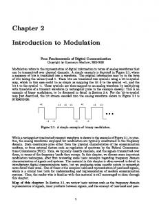
definition of u. Figure 1, for an arbitrary probability density function f(x), shows equation (1) graphically. The gaussian (normal), Rayleigh, exponential, and Laplacian distributions are among the examples of the asymptotically exponential distributions. All of these distributions. may be ~pp.roximated by Equation (1) in the vicinity of u. How far from the vicinity of u one may move depends of course on the actual underlying distribution and the particular point (u) one expands . about. As an example Figure 2 compares the exponential approximation to the actual probability of exceedance of x, P e, for a gaussian density function. Here n has been arbitrarily chosen as 100. The actual probability Pe and its exponential approximation are then matched at Pe = 10-2. It is readily shown that the point Un about which one expands, is 2.32, "and an =2.68.

483 From the collection of the Computer History Museum (www.computerhistory.org)

484

Spring Joint Computer Conference, 1968

x

JLn Xo Fig-lire 1 - Exponential approximation to probability of error

Comparing the probability of exceedance Pe for the actual gaussIan and its exponential approximation, as plotted in Figure 2, it is apparent that the two are within 25% of one another at Pe = 10-3 and differ by 50% at Pe= 10-4 • This then points up the significance of the extremal statistics approach: if one is interested in estimating small probabilities of error, say of the order of 10-3 or 10-4 , it may be possible instead to first estimate much higher probabilities, say 10-2 in the example of Figure 2~ If the exponential approximation is valid one should then be able to extrapolate down to the desired probability. Instead of the usual number of samples required to estimate Pe, say 1O/Pe, one can then work with a much smaller number n.

There is of course one major problem, however. Since the underlying density function f(x) is in general unknown, or difficult to evaluate in the complex systems of interest to us, the two parameters an and Un are unknown as well, and must be estimated, In the next section we discuss various ways of estimating an and Un, and results of computer runs for two simple density functions, the gaussian and the exponential. The results are quite encouraging: even with additional samples needed to estimate an and Un, one can still save at least an order of magnitude in the total number of samples required to estimate a given probability of error the traditional way. I.n the finai ~ec~ion, we discuss the computer simulation of two specific feedback communications systems for which probabilities of error have been estimated quite successfully using extremal statistics. (One of these systems is an example of one for which actual calculations or probabilities of error are quite difficult to make. In the example shown only bounds .on the error have been obtained and the simulation results check these quite closely.)

Extimation of extremal parameters We discuss in this section the use of extremal statistics to estimate small probabilities of error in the case of two known distributions, the exponential and the gaussian. The problem here is twofold: to first estimate the extremal parameters an and U m then to determine, using these estimates, how well the actual probabilities at the tails are estimated. The exponential density function normalized to unit variance is given by f(x) = e-Xu(x)

2 1.=10n GAUSSIAN APPROX:

an= 2.68 POn= 2.32

10-4

10-5L----L----........L.----~4-...,.

2

:3

Figure 2 - Exponential approximation to gaussian statistics

(2)

u(x) the unit step function, while the gaussian density function, again normalized to unit variance, is of course given by f(x) = _1_ V2.'TT

e-x2/2

(3)

One would expect rather good estimates of the probability at the tail for the exponential density function since it is already in the asymptotic form of equation (1). In the gaussian case, as pointed out in the previous section and as illustrated for one case in Figure 2, it is theoretically possible to extrapolate as much as two orders of magnitude away from the starting point 1In before the quadratic exponential behavior of the gaussian function takes over and produces significant deviations away from the linear exponential behavior of extremal statistics.

From the collection of the Computer History Museum (www.computerhistory.org)

Extremai Statistics in Computer Simuiation The actuaJ experimental behavior of the exponential approximation depends critically on the estimation of the two parameters an and Un- To determine these we . use the fact, as demonstrated by Gumbel, l that they are intimately connected to the asymptotic statistics of the extrema (maxima) of the random variable x. Specifically, if one generates n independent samples of x the probability density function of the largest (maximum), x rn , of the n samples is asymptotically (n~oo) given by ~

puter simulation involved would thus be nN = 104. The resultant output samples would be grouped into N = 10 groups of n = 103 samples each. The largest sample, Xh in each group would then provide N = 10 samples with wh~~h to estimate an and Un'

nN=10 4 SAMPLESOFX 111111111···111···111···111

x nN

XI n

REGROUP iNTO N=iO IN GROUpS n=103 EACH

P n = an exp [-y-e- v ] y == an[xrn-un]

485

n. n

n

,'Oii7iiiI "1iii"iiI ,'mm" '" "'imiI" I

2

3

10

(4) LET X i BE LARGEST SAMPLE IN EACH GROUP

Equation (4) is found to be valid for a wide class of density possessing exponential behavior at the density functions posse~sing exponential behavior at the tails, with the exponential, gaussian, and Rayleigh functions typical examples. From Equation (4) it is readily shown that un(n~oo) is a measure of the mode of Pn(xm> , while a.!.(n~oo) is a

n

measure of the dispersion. Specifically, one finds, using Equation (4), that 1

V6

-=-(J"rn a 1T

(5)

and (6)

Here (J"rn is the standard deviation of the maximum (extremal) values, xrn , of x, E(xrn ) the expected value of these maxima, and 'Y = 0.5772 is just Euler's constant. ~t is thus apparent. that to estimate an and Un one must first ensure n > > 1 (This is why Equation (1) is applicable to the tails of density functions, where Pe < < 1), and then generate sufficient samples of the random variable x under test to measure their statistical properties. If N samples of the largest value of x in a group of n are to be made available this implies repeating the experiment nN times in all. It is the total number nN that is to be compared to the usual number 10/Pe •

From !he form of Equations (5) and (6) one would expect that for n and N large enough, good approximations to an and Un would be obtained by averaging appropriately over the N samples of the maxima available. As noted later this was in fact found to be the simplest and most accurate procedure in actual experimentation with the computer. This estimation procedure is portrayed in Figure 3. There, as an example, n = 103 and N = 10 are chosen. ~he total number of independent samples or repeats of the com-

Figure 3 - Estimation of a and Un

There is a tradeoff possible between nand N, given the fixed number of repetitions nN. Thus decreasing n decreases the range over which one would theoretically expect the asymptotic exponential approximation to hold (assuming perfect knowledge of an and un), but allows better estimation of an and Un as N increases. Some analysis of the optimum choice of n and N has been carried in a recently completed doctorial thesis.4 In the actual computer simulations carried out n was taken as 500, N = 20, so that a total of 10,000 actual repetitions of the different experiments tried were performed. Normally this would provide relatively accurate estimation of probabilities of error as low as 10-3 • We were interested in extending the estimation to 10-4 and 10-5 • As noted previously, an obvious initial estimate for a is to replace (J"rn in Equation (5) by the sample standard deviation s, using the N = 20 samples available of the extrema. Similarly a first estimate for u is to replace E(xrn ) in Equation (6) by the sample mean ·'Xrn (again using the 20 extremum samples). (These are the procedures suggested in Figure 3.) Although the sample standard deviation is in general a rather poor estimator of the statistical stand~rd deviation [var (S2) = 2(J"~JN· for gaussian statistics] the experimental results obtained were surprising~y _go