Extreme Long-time Dynamic Monte Carlo Simulations

arXiv:cond-mat/0207405v1 [cond-mat.stat-mech] 16 Jul 2002

International Journal of Modern Physics C cfWorld Scientific Publishing Company

Extreme Long-time Dynamic Monte Carlo Simulations for Metastable Decay in the d=3 Ising Ferromagnet

Miroslav Kolesik Optical Sciences Center University of Arizona Tucson, Arizona 85721, U.S.A. E-mail: [email protected] M.A. Novotny Department of Physics and Astronomy Mississippi State University P.O. Box 5167 Mississippi State, Mississippi, 39762-5167, U.S.A. E-mail: [email protected] Per Arne Rikvold Department of Physics and Center for Materials Research and Technology and School of Computational Science and Information Technology Florida State University Tallahassee, Florida 32306-4350, U.S.A. E-mail: [email protected]

Received (received date) Revised (revised date)

We study the extreme long-time behavior of the metastable phase of the threedimensional Ising model with Glauber dynamics in an applied magnetic field and at a temperature below the critical temperature. For these simulations we use the advanced simulation method of projective dynamics. The algorithm is described in detail, together with its application to the escape from the metastable state. Our results for the field dependence of the metastable lifetime are in good agreement with theoretical expectations and span more than fifty decades in time. Keywords: Metastability, Ising, Dynamic Monte Carlo, Time Scales

1. Introduction One of the most difficult and most important problems in simulation in the sciences and engineering is that of disparate time and length scales. The difficulty in the time-scale problem is the wide separation between the time scales of microscopic and macroscopic phenomena. Consider a simulation to study the time dependence of a nanoscale ferromagnetic particle or thin film using a dynamic Monte Carlo

procedure. The microscopic time scale corresponds approximately to an inverse phonon frequency, or about 10−13 seconds. The time over which simulations need to be performed corresponds to the time scale over which random thermal events change the direction of the magnetization. For data recording applications this corresponds to the time over which data written on magnetic recording media should be stored: years to decades. For studies in paleomagnetism, the time scales to be simulated are millions of years. Bridging such disparate time scales obviously requires faster-than-real-time simulation algorithms. In this paper we present in detail a method to perform simulations that extend over extremely long times for the short-ranged ferromagnetic three-dimensional Ising model with Glauber dynamics at a temperature below the critical temperature. The method can be generalized to other dimensions, to other models with discrete state spaces, and to other dynamics. The fact that many, many decades in time can be obtained in computer simulations of metastable decay of the d = 3 Ising ferromagnet shows that the required faster-than-real-time simulations are indeed feasible. The remainder of this paper is organized as follows. The general features of metastable decay in kinetic Ising models are discussed in Sec. 2. The projective dynamics method of accelerated dynamic Monte Carlo simulation is briefly described in Sec. 3. Our numerical results are presented in Sec. 4, while Sec. 5 is devoted to a brief discussion and conclusions. 2. Metastability and the Ising Model The Hamiltonian of the Ising model is given by X X σi . σi σj − H H = −J hi,ji

(1)

i

In Eq. (1), J is the nearest-neighbor exchange interaction which we take as ferromagnetic and for simplicity of notation set equal to unity, H is the applied external magnetic field, the first sum is over all nearest-neighbor pairs of spins on a ddimensional hypercubic lattice, and the second sum is over all N = Ld spins. Each spin can take two values, denoted by ‘up’ and ‘down’ or σ = ±1. We impose periodic boundary conditions. (The projective dynamics method could also be used with other boundary conditions, but it is simplest for periodic boundary conditions.) The temperature is chosen below the critical temperature Tc (in this work, 0.6Tc), so that in zero field the system has two degenerate, ordered phases with magnetizations near ±1. In an applied field, the ordered phase in which the spins are aligned opposite to the field becomes metastable. The value of the critical temperature used here corresponds to J/kB Tc = 0.22165, as obtained in high-precision Monte Carlo simulations.1,2 The dynamic used corresponds to one derived from consideration of quantum spin 21 particles interacting with a fermionic heat bath. In certain limits, it has been

shown3 that this corresponds to the dynamic: 1) a spin is chosen at random from among all N spins; 2) the spin is flipped with the Glauber4 transition probability p=

exp(−βEnew ) 1 = , exp(−βEnew ) + exp(−βEold ) 1 + exp [β (Enew − Eold )]

(2)

where β = 1/(kB T ) and kB is Boltzmann’s constant, the energy of the current configuration is Eold , and the energy of the configuration obtained if the chosen spin is flipped is Enew . One cycle through these two steps, whether or not a new configuration is obtained, is one Monte Carlo step. Time is measured in units of N such cycles, which is called one Monte Carlo step per spin (MCSS). Note that the dynamic described above corresponds to a particular physical dynamic, and that the time dependence of the system with this dynamic is the quantity of physical interest. Consequently, the dynamic cannot be changed by the simulation algorithm. To implement a faster-than-real-time simulation the dynamic can only be implemented on a computer in a more intelligent fashion. The restriction against changing the dynamic means that common advanced simulation techniques such as cluster algorithms, multicanonical methods, and simulated tempering, cannot be used since they all change the underlying dynamic of the system. Also note the restriction to randomly (rather than sequentially) picking the spin in the first step. In some cases it has been shown that dynamic results differ between sequential and random updates. In particular, the prefactor in metastable decay has been shown in some cases to depend on whether the spin is chosen randomly or sequentially.5,6 We use random updates for two reasons. First and foremost this procedure corresponds to the dynamic obtained from coupling the quantum system to the heat bath. Second, advanced dynamic simulation algorithms, such as projective dynamics, are easier to implement in the random update scheme. We wish to study the lifetime of the metastable phase of the simple cubic Ising model with periodic boundary conditions. The system is initially prepared with all spins up (all σ = 1), and the applied field H is negative. Starting from this metastable initial state, we measure the metastable lifetime τ as the time when the magnetization first attains or crosses a pre-determined stopping value, mstop (i.e., the first-passage time to mstop ). The particular value of mstop is not very important, as long as it is chosen between the value corresponding to the saddle point and the value corresponding to the equilibrium state, and τ does not have a substantial contribution from the time required to slide from the saddle point toward the equilibrium state. In this work, we make the customary choice of mstop = 0. The average lifetime, hτ i, is obtained by averaging τ over many realizations, each of which uses a different random number sequence. The dependence of hτ i on T and H is of central physical importance. 3. Projective Dynamics for the d = 3 Ising Model The slow-forcing method we apply to study the extremely long-lived metastable states was described in detail in Refs. 7,8,9,10 For the sake of completeness, we de-

scribe briefly the main features of the approach here. It was designed for simulation of the escape from a metastable state with a very long lifetime. Its core is based on an n-fold way simulation algorithm10,11,12,13 that preserves the prescribed local Monte Carlo dynamic but eliminates all unsuccessful attempted updates. This method is suitable for measuring lifetimes many orders of magnitude longer than those accessible by conventional algorithms. To extend the reach of simulations to even radically longer lifetimes, the n-fold way method has to be augmented in two ways. First, we have observed and proven that the mean lifetime of a metastable state can be calculated from the so-called projected growth and shrinkage rates of the stable phase within the metastable phase.9 To obtain an exact answer for the mean lifetime, one of course needs to know the growth and shrinkage rates exactly as functions of the total volume fraction of the stable-phase regions. Since we do not have this exact information, we have to resort to measuring the rates. It can be shown that the n-fold way simulation itself samples these rates in an appropriate way and can thus be used to obtain estimates of the growth and shrinkage rates as functions of the total volume fraction of the stable phase.9,10 However, although such an approach provides certain advantages, for example in studying the size dependence of the mean lifetime,7 it does not actually extend the regime of measurable lifetimes. To achieve that, we make the second departure from the straightforward simulation approach. Namely, we modify the a-priori part of the Monte Carlo transition rates in such a way that the volume of the stable phase is not allowed to decrease below a certain value. This value is gradually increased during the simulation to force the system from its metastable free-energy minimum over the barrier into the stable phase. We call this minimal allowed volume of the stable phase a forcing constraint in accordance with its effect on the dynamics of the system. The simulation is initialized with the forcing constraint equal to zero and an n-fold way simulation is performed while the constraint is increased very slowly. This way, the system samples configurations along the path of the escape from the metastable free-energy minimum with the correct weights for measuring concentrations of spins in different classes. These spin classes and the corresponding energy changes are shown in Table 1. After the system reaches the states sufficiently close to the top of the free-energy barrier and overcomes it, it converges quickly toward the true stable state. At this stage the forcing constraint becomes irrelevant because of the relative rapidity of the last escape stage. Naturally, the duration of the forced escape has nothing to do with the true metastable lifetime, because we have modified the dynamic in a radical way. However, during the multiple repetitions of the forced escapes, we gather sufficient statistics to estimate the growth and shrinkage rates along the whole escape path, which in turn are used to calculate an estimate of the actual mean lifetime. Naturally, the question arises of whether the forced, modified dynamic leaves the growth and shrinkage rates unaltered. As may be expected, the rates and the corresponding mean lifetime actually do depend on the forcing speed. However, with decreasing forcing speed they converge to their slow-forcing limit.9,10 This convergence is sufficiently fast to obtain estimates of

Table 1. The 14 energy classes for the simple cubic Ising lattice. Class Number 1 2 3 4 5 6 7 8 9 10 11 12 13 14

Spin ↑ ↑ ↑ ↑ ↑ ↑ ↑ ↓ ↓ ↓ ↓ ↓ ↓ ↓

Number of nn spins up 6 5 4 3 2 1 0 6 5 4 3 2 1 0

Enew − Eold −2H + 12J −2H + 8J −2H + 4J −2H −2H − 4J −2H − 8J −2H − 12J +2H − 12J +2H − 8J +2H − 4J +2H +2H + 4J +2H + 8J +2H + 12J

exceedingly long lifetimes. While we have no formal proof for the convergence, it is possible to see intuitively why it works. During the early stages of the forced escape, the sampled configurations and values of the growth and shrinkage rates are close to the states of the unperturbed escape provided the great majority of the Monte Carlo moves are not constrained. The sufficiently rare invocation of the constrained dynamic rule can be achieved at an appropriately slow forcing rate. Close to and behind the free-energy barrier, the evolution is rapid, and the volume of the stable phase grows faster than the progress of the forcing constraint. Therefore, at this stage the system follows its natural non-equilibrium path toward the stable phase. It is mainly this stage which requires one to repeat the forced escape many times in order to gather sufficient statistics for the non-equilibrium portion of the escape path. Before discussing our numerical results in Sec. 4, we present a summary of the formulas needed to interpret the simulation data. Again, the reader is referred to the above references for details. The growth and shrinkage rates in the slowforcing limit are defined in terms of the average class populations and Monte Carlo dynamic transition rates. While the latter are given or specified by the simulated system [Eq. (2)], the meaning of the former has to be made more accurate. These class populations are normalized probabilities for the occurrence of spins with the corresponding nearest-neighbor configurations. The average is taken with respect to the ensemble generated by an unperturbed escape from the metastable state. The sampling during the repeated forced escapes provides us with an estimate of the growth rates g(n) and shrinkage rates s(n) for a system with n spins down, g(n) =

6 X a=0

′

c↑a (n) p↑↓ a , s(n) =

6 X

c↓a (n) p↓↑ a ,

(3)

a=0

where pσσ are the prescribed Monte Carlo spin-flip transition rates from σ to σ ′ for a

spins with a nearest neighbors up, and cσa (n) stand for the spin-class populations which are sampled in the process. The growth and shrinkage rates, g(n) and s(n), have to be obtained for all n between zero and nstop ≈ nstable that corresponds to the stable-phase magnetization. As mentioned above, the precise setting of nstop is irrelevant as long as it is well beyond the top of the free-energy barrier separating the metastable phase from the stable phase. The mean lifetime is then given by the formula nstop

hτ i =

X n=0

h(n) , h(n − 1) =

L−d + s(n)h(n) , g(n − 1)

(4)

where h(n) is the cumulative residence time in the state with n spins down. As noted before, this expression is formally exact if the growth and shrinkage rates in the slow-forcing limit could be obtained. It represents a sum of the residence times h(n) in the configurations with n spins down. The values of h(n) make up a histogram that is peaked sharply around the value of n corresponding to the magnetization of the metastable phase. Our approximation consists in replacing g(n) and s(n) by their corresponding estimates obtained at a finite forcing rate. 4. Results We have performed a series of simulations using both the direct n-fold method and the forced-escape method to obtain the mean lifetime of the metastable state of the three-dimensional ferromagnetic Ising model with Glauber dynamic at a temperature of 0.6Tc (this is about 11% above the roughening temperature22 ). Below we present results for the system size of Ld = 163 and a range of external fields. The data acquired by the forced-escape method for a set of chosen strengths of the external field were utilized to obtain estimates of the spin-class populations and of the growth and shrinkage rates at other values of the external field by straightforward interpolation and extrapolation. Figure 1 shows the global picture of the mean lifetime as a function of the external field that drives the system toward its true equilibrium state. The lifetime data are plotted on a logarithmic scale versus 1/|H|d−1 = 1/H 2 , so that data in both the single-droplet and multidroplet decay regimes should show up as approximately straight lines. (Different regimes of the magnetization reversal and the rationale for this plotting method are described in Refs. 5,6,14,15,16,17 ) The straight portion of the graph in Fig. 1 corresponds to the single-droplet regime, in which the escape from metastability is triggered by a single critical droplet of the stable phase. The bend in the strong-field portion of the curve is the cross-over to the multidroplet regime, in which many supercritical droplets exist by the time the system reaches the cut-off magnetization (the corresponding field is known as ”the dynamic spinodal” 5,6 ). The gradual bend in the weak-field region is due to the cross-over into the coexistence regime, which is characterized by a critical fluctuation comparable in size with the system itself.

Note the exceedingly long lifetimes our approach enables us to estimate. (To put the range of time scales into perspective, we note that the age of the universe, measured in femtoseconds, is about 1033 .) By itself, the fact that we can reach almost to the coexistence regime demonstrates the power of the method. Standard n-fold way simulation results are also included in the figure to contrast the corresponding orders of magnitude. To make the details at stronger fields discernible, we present in Fig. 2 a blow-up of the lower-left portion of Fig. 1. There one can see that direct lifetime measurements are perfectly reproduced by the slow-forcing escape simulations, even though the latter were performed only for a limited set of external field values. Naturally, with estimated lifetimes this long, and in the absence of direct comparison with other computational methods, the question arises of how accurate our estimates actually are. This is, of course, a difficult question to answer. One way to approach this problem is to look at the theoretically predicted behavior of the mean lifetime as a function of the external field strength. Namely, the dominant field dependence is expected to be universal, having the form of an exponential modified by a field-dependent prefactor. The droplet theory of metastable decay predicts a characteristic behavior for the effective slopes of the logarithm of the mean lifetime as plotted in Figs. 1 and 2,5,6 Λeff =

d ln hτ i = λ|H|d−1 + Λ , d(1/|H|d−1 )

(5)

where the values of λ and Λ depend on the magnetization reversal regime [singledroplet (SD) or multidroplet (MD)] and on the microscopic dynamic. In three dimensions and with a dynamic with updates at randomly chosen sites as used here, field-theoretical calculations18 predict for the single-droplet regime λSD = −1/6 and ΛSD = βΞ(T ), where Ξ(T ) is the field-independent part of the free energy of the critical droplet.5,6 In the multidroplet regime, the field-theoretical results, combined with the Kolmogorov-Johnson-Mehl-Avrami theory of metastable decay in large systems,5,19,20 yield λMD = +1/3 and ΛMD = βΞ(T )/(d + 1) = βΞ(T )/4. From the droplet theory one obtains Ξ(T ) (here given specifically for three dimensions) as Ξ(T ) ≈ Ω3 σ 3 /m2 .5,6 Here σ(T ) is the equilibrium surface tension of an interface parallel to one of the lattice symmetry directions, separating the positively and negatively magnetized phases, and m(T ) is the spontaneous equilibrium magnetization in zero field. The quantity Ω3 (T ) is a shape factor which interpolates smoothly between 8 for cubic droplets in the low-temperature limit and 4π/3 for spherical droplets at higher temperatures, and it could in principle be obtained by a Wulff construction with the full, anisotropic surface tension.5,21 Since the latter is not available, we simply use the extreme values of Ω3 to obtain lower and upper bounds on βΞ(0.6Tc ). For this purpose we use estimates for the surface tension and magnetization obtained from high-precision equilibrium Monte Carlo simulations, σ(0.6Tc )/J ≈ 1.536,22 and m(0.6Tc) ≈ 0.971.23 The resulting approximate lower and upper bounds on βΞ(0.6Tc ) are 5.948 and 11.359, respectively.

The quantities that enter into Λeff are very sensitive to sampling errors, and they are not easy to obtain, even from direct simulations when such are feasible. It is therefore a good test of our results to evaluate the effective slopes to see whether the expected characteristic behaviors are recovered. In Fig. 3 we have plotted Λeff vs |H|d−1 = H 2 , where the continuous curve is obtained by numerical differentiation of the mean lifetimes, which in turn were calculated from the interpolated and extrapolated class-population data. We see that the main features of the expected cross-over between the multidroplet and single-droplet regimes is well pronounced, as is the rapid decrease of Λeff for very weak fields that corresponds to the cross-over to the coexistence regime (see below). However, our effective slope curve exhibits modulations which are clearly artifacts of the interpolation procedure. These modulations prevent us from determining the simulated values of λSD and λMD . Instead, we have placed straight lines with the theoretically predicted values of λSD and λMD , so as to independently match Λeff in the single-droplet and multidroplet regimes reasonably by eye. The resulting intercepts with the vertical axis give estimates ΛSD = βΞ(0.6Tc ) ≈ 6.6 and ΛMD ≈ 1.8. Thus, our estimate for βΞ(0.6Tc ) lies between the lower and upper bounds obtained from droplet theory. As it lies closer to the lower bound, our simulations may indicate that the average critical droplet is closer to spherical than to cubic. Furthermore, the ratio ΛSD /ΛMD ≈ 3.7, in reasonable agreement with its expected value of 4. Another characteristic feature of Fig. 3 is the steep drop in Λeff for weak fields. At the field where this drop sets in (known as ”the thermodynamic spinodal field”,5,6 HTHSP ), the free energy of the critical droplet equals that of a slab of the same volume, which spans the system in two dimensions. This field can also be obtained analytically by droplet-theoretical arguments 24,25 as (given specifically for three p dimensions) HTHSP ≈ σ 3Ω3 /2/(mL), yielding lower and upper bounds at T = 0.6Tc of 0.2478 and 0.3425, respectively. The corresponding range for H 2 is shown in Fig. 3 as a thick, horizontal bar above the Λeff curve. The agreement between our simulation results and this theoretical prediction is also very good. The above considerations give us a feeling for how accurate the forced-escape lifetime estimates are: the method provides sufficiently reliable results for the lifetimes themselves, but the coarse sampling of the external field used in the present work prevents us from taking numerical derivatives of the lifetime with sufficient accuracy to reliably estimate their dependence on the applied field. To improve the effective-slope estimates, it would not only be necessary to perform the forcedescape simulations over a denser set of field strengths, but also to increase the number of simulated escapes at each field strength. To increase the accuracy of the slope determination in the multidroplet regime, it would also be necessary to use larger systems to increase the range of fields corresponding to that regime. Nevertheless, we find the agreement with the theoretical predictions of our estimates for ΛSD , ΛMD , and the cross-over field to the weak-field coexistence regime quite encouraging.

5. Discussion and Conclusions We have described the method of projective dynamics with slow forcing and applied it to the long-time simulation of the metastable lifetime of the simple-cubic Ising model with the Glauber dynamic. We have obtained the lifetime corresponding to the dynamic Monte Carlo simulation over more than fifty orders of magnitude without changing the dynamics of the model! From the dependence of the lifetime on the applied field we are able to identify different regimes of decay for the model.5,6 The results thus far are good enough to see the expected dependence of the lifetime on the applied field. This slow-forcing projective dynamics method can also be used in other simulations of discrete-state models to bridge widely disparate time scales. Acknowledgments Useful discussions with S.J. Mitchell are acknowledged. This research was funded partly the the U.S. National Science Foundation through grants No. DMR-9871455 and DMR-0120310. M.K. was partly supported by the Slovak Grant Agency through Grant No. 2/7174/20. 1. 2. 3. 4. 5. 6. 7.

8. 9. 10. 11. 12. 13. 14. 15. 16. 17. 18. 19.

C.F. Baillie, R. Gupta, K.A. Hawick, and G.S. Pawley, Phys. Rev. B 45, 10438 (1992). A.L. Talapov and H.W.J. Bl¨ ote, J. Phys. A: Math. Gen. 29, 5727 (1996). Ph.A. Martin, J. Stat. Phys. 16, 149 (1977). R.J. Glauber, J. Math. Phys. 4, 294 (1963). P.A. Rikvold and B.M. Gorman, in Annual Reviews of Computational Physics I, edited by D. Stauffer (World Scientific, Singapore, 1994), p. 149, and references therein. P.A. Rikvold, H. Tomita, S. Miyashita, and S.W. Sides, Phys. Rev. E 49, 5080 (1994). M. Kolesik, M.A. Novotny, P.A. Rikvold, and D.M. Townsley, in: Computer Simulation Studies in Condensed Matter Physics X, edited by D.P. Landau, K.K. Mon, and H.-B. Sch¨ uttler (Springer, Berlin, 1998) p. 246. M. Kolesik, M.A. Novotny, and P.A. Rikvold, Phys. Rev. Lett. 80, 3384 (1998). M.A. Novotny, M. Kolesik, and P.A. Rikvold, Comput. Phys. Commun. 121-122, 330 (1999). M.A. Novotny, in Annual Reviews of Computational Physics IX, edited by D. Stauffer (World Scientific, Singapore, 2001), p. 153. A.B. Bortz, M.H. Kalos, and J.L. Lebowitz, J. Comput. Phys. 17, 10 (1975). M.A. Novotny, Computers in Physics 9, 26 (1995). M.A. Novotny, Phys. Rev. Lett. 74, 1 (1995); Erratum 75, 1424 (1995). H.L. Richards, S.W. Sides, M.A. Novotny, and P.A. Rikvold, J. Magn. Magn. Mater. 150, 37 (1995). H.L. Richards, S.W. Sides, M.A. Novotny, and P.A. Rikvold, J. Appl. Phys. 79, 5479 (1996). H.L. Richards, M.A. Novotny, and P.A. Rikvold, Phys. Rev. B 54, 4113 (1996). H.L. Richards, M. Kolesik, P.-A. Lindg˚ ard, P.A. Rikvold, and M.A. Novotny, Phys. Rev. B 55, 11521 (1997). N.J. G¨ unther, D.A. Nicole, and D.J. Wallace, J. Phys. A 13, 1755 (1980). A.N. Kolmogorov, Bull. Acad. Sci. USSR, Phys. Ser. 1, 355 (1937); W.A. Johnson and R.F. Mehl, Trans. Am. Inst. Mining and Metallurgical Engineers 135, 416 (1939); M. Avrami, J. Chem. Phys. 7, 1103 (1939); M. Avrami, J. Chem. Phys. 8, 212 (1940); M. Avrami, J. Chem. Phys. 9, 177 (1941).

20. R.A. Ramos, P.A. Rikvold, and M.A. Novotny, Phys. Rev. B 59, 9053 (1999). 21. C.C.A. G¨ unther, P.A. Rikvold, and M.A. Novotny, Physica A 212, 194 (1994). 22. M. Hasenbusch and K. Pinn, Physica A 203, 189 (1994). Our value for σ(0.6T c) was obtained by linear interpolation from Table VII of this reference. (Note that our σ corresponds to these authors’ σ/β .) 23. Our value for m(0.6Tc ) was obtained from Fig. 1 of Ref. 2 , together with Eq. (10) from the same reference. 24. K. Leung and R.K.P. Zia, J. Phys. A 23, 4593 (1990). 25. J. Lee, M.A. Novotny, and P.A. Rikvold, Phys. Rev. E 52, 356 (1995).

60

10

48

mean lifetime

10

36

10

24

10

12

10

0

10

0.0

10.0

20.0

30.0

40.0

2

1/H

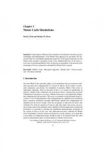
Fig. 1. The average lifetime hτ i in units of Monte Carlo steps per spin (MCSS) for the d = 3 ferromagnetic Ising model with Glauber dynamics at a temperature of 0.6Tc . The lifetime is shown on a logarithmic scale as a function of 1/H 2 . Note the extremely long lifetimes obtained in this computer simulation. The cross symbols indicate external field values for which the growth and shrinkage rates were measured, while the full curve was calculated from interpolated and extrapolated rates. The filled squares in the lower left-hand (strong field, short time) corner of the figure represent standard n-fold way simulations. A magnified view of this region is shown in Fig. 2.

8

10

mean lifetime

6

10

4

10

2

10

0

10

0.0

1.0

2.0

3.0

4.0

2

1/H

Fig. 2. The magnified region of the relatively short lifetimes from Fig. 1. In the lower part of this region, direct n-fold way simulations are feasible. The corresponding direct simulation estimates are indicated by filled squares. As in Fig. 1, the crosses represent slow-forcing simulations, and the solid curve was calculated from interpolated rates.

Λeff 2 6.6 − H /6 2 1.8 + H /3

6

Λeff

4

2

0

0

0.2

0.4

0.6 H

0.8

1

2

Fig. 3. Numerical estimate of the effective slope Λeff , shown vs H 2 . The thick solid curve is obtained by numerical differentiation of the curve shown in Fig. 1. The thin solid and dashed straight lines are theoretical predictions for the single-droplet and multidroplet regimes, respectively, with y-intercepts fitted as described in the text. The horizontal bar in the upper left corner represents the theoretical range of H 2 for the cross-over to the coexistence regime.