A. Agnes, F. Maloberti, G. Martini: "Improved Chopper Stabilized Amplifier for Offset and 1/f Noise Cancellation"; 13th IEEE International Conference on Electronics, Circuits and Systems, ICECS 2006, Nice, 10-‐13 December 2006, pp. 529-‐532. ©20xx IEEE. Personal use of this material is permitted. However, permission to reprint/republish this material for advertising or promotional purposes or for creating new collective works for resale or redistribution to servers or lists, or to reuse any copyrighted component of this work in other works must be obtained from the IEEE.
Improved Chopper Stabilized Amplifier for Offset and 1/f Noise Cancellation A. Agnes, F. Maloberti, G. Martini Department of Electronics, University of Pavia Via Ferrata, 1, 27100 Pavia, Italy Email:
[email protected],
[email protected],
[email protected] Abstract— The limits of the conventional chopper stabilization technique for cancelling the 1/f noise are studied theoretically and with simulations. The expected replicas of the 1/f noise at the chopping frequency and its multiples are attenuated by a modified chopping control. Simulation done using records of real 1/f noise outputs show that the spectrum of the signal does not change but 1/f replicas are reduced by more than 40 dB. The required circuit for the generation of the chopping signal is also described. The resulting overhead with respect to conventional solutions is negligible and fully acceptable.
I. I NTRODUCTION Many instrumentation applications require using amplifiers with very high gain and virtually zero offset and 1/f noise. The used solutions are nested amplifiers like the one shown in Fig. 1 with the first amplifier, A1 , using a cancellation technique. The scheme obtains a low-frequency gain A0 = A2 + A1 A2 and cancels the offset and the 1/f noise of A1 using extra blocks before and after the amplifier as generically indicated in the Fig. 1. The offset and 1/f noise of A2 are referred at the input attenuated by A0 /A2 The methods used for obtaining the cancellation are two: the auto-zero [1] and the chopper stabilization [2]. The former method is sampled-data as it requires a time-slot during which the amplifier is not used: it is connected in some configuration for making available a sample of the input referred error (offset plus noise) or its amplification. The signal is stored in a capacitance for a successive cancellation. The chopper stabilization technique uses a double synchronous modulation of the input that does not alter the spectrum of the signal and a single modulation of input referred error that is brought to high frequency, out of the band of interest. The auto-zero and the chopper stabilization have advantages and disadvantages as it will be studied below in some details. This paper proposes a chopping technique that significantly reduces the key disadvantage of the second method and makes it
Vin (t)
Σ
M1 q(t)
Σ
n(t)
A1
M2
A2
Vout (t)
Vout1(t) + x(t)
q(t)
Fig. 1. Generic Scheme of a nested amplifier with offset and 1/f cancellation.
1-4244-0395-2/06/$20.00 ©2006 IEEE.
529
preferable for integrated solutions that does not admit external components. Theoretical studies and simulations result prove the benefit of the proposed approach. II. S YSTEM M ODEL A simple model of output noise due to low frequency noise of the amplifier A1 placed between the modulator and the demodulator, it is shown in Fig. 1, where q (t) is the modulating signal, Vout and Vout1 are the output signals, at the nodes indicated, due to the input signal Vin without any noise, and the Stochastic Process (SP) n (t) is the (low frequency) noise of A1 referred at its input; the mean value of n (t), E {n (t)} = e, is the input offset voltage of A1 . Vin = 0 is assumed, so that only the noise behavior of the circuit is considered. The output of the demodulator M 2 is viewed as the sum of Vout1 , that is the contribution of Vin and vanishes for Vin = 0, and of the noise contribution x (t). Within the paper only the noise term x (t) is considered, and any Power Spectral Density (PSD) is assumed to be one-sided unless otherwise staded. No input offset voltage, i.e. e = 0, and an input referred noise n (t) with PSD1 of the form: Sn (f ) =
K f
(1)
is assumed. By writing (1), n (t) is taken as, at least, a Wide Sense Stationary (WSS) SP, also if it is not so, as pointed out by Keshner [3]; n (t) can be in practice considered as being WSS with PSD given by (1). By naming Rn (τ ) the Autocorrelation Function (AF) corresponding to (1), from the system model in Fig. 1, assuming A1 = 1 for the sake of simplicity, the output noise x (t) results from the intermodulation (product) between n (t) and the modulating signal q (t), i.e. x (t) = n (t) q (t). The modulation is usually implemented by switching, so that the modulating signal is usually a ±1 square wave with given (fixed) frequency f0 . With this kind of q (t), the 1/f PSD is removed from the baseband and shifted to f0 and its odd harmonics, appearing mainly as 1/ | f − (2i + 1) f0 | PSD. Our proposal is to use a random modulating signal with proper PSD to substantially reduce noise peaking. Two cases are discussed in the following. 1 The 1/f frequency dependence of the single-sided PSD in (1) comes from the actual 1/|f | frequency dependence of the corresponding doublesided PSD.
of q (t), so that the variance of the (non stationary) SP ϕ (t) is σϕ2 = c1 t. The PSD corresponding to (7) is:
A. Square wave modulation at constant frequency By assuming a ±1 square wave q (t), as usual: ∞ 4 ! sin [(2i + 1) 2πf0 t] π i=0 (2i + 1)
(2)
for constant chopping frequency f0 the SP x (t) is cyclostationary with the same fundamental frequency f0 , i.e its AF function can be written as [4]: Rx (t1 , t2 ) = E {x (t1 ) x (t2 )} = q (t1 ) q (t2 ) Rn (τ ) ∞ ! = Rx,i (τ ) ej2πif0 t (3) i=−∞
where τ = t1 −t2 and t = (t1 + t2 ) /2. Each term multiplying the i−th exponential term in the last line of (3) is called Cyclic Autocorrelation Function (CAF) of i − th order; in practice, if the output signal is not multiplied by any other clock with frequency i f0 and coherent with q (t), only the stationary part of the AF is of concern. For q (t) given by (2) the stationary part of (3) is: ∞ 16 ! cos [(2 i + 1) 2 πf0 t] Rn (τ ) Rx,0 (τ ) = 2 2 π i=0 2 (2 i + 1)
(4)
From (1) and from convolution theorem of Fourier transform, following the procedure outlined in [5] the PSD corresponding to (4) is obtained as: ∞ Ci K ! Sx,0 (f ) = 4 i=−∞ | f − (2 i + 1) f0 | 2
Sq (f ) =
∞ γ 8 ! 4 3 2 π i=−∞ γ (2 i + 1) + [f − (2 i + 1) f0 ]2
Rx (τ ) = E {x (t1 ) x (t2 )} = Rq (τ ) Rn (τ )
2
B. Square wave with large linewidth To avoid noise peaking around the modulation frequency and its odd harmonics some randomization of the modulating square wave can be used. As an example of “randomized” clock, a very noisy clock is considered. Real clock generators are affected mainly by phase noise that is usually well described by a Random Walk (RW) [6] phase ϕ (t) added to the linear phase 2 πf0 t. Such a noisy ±1 square wave can be written as: ∞ 4 ! sin [(2 i + 1) (2 πf0 t + ϕ (t))] (6) q (t) = π i=0 (2 i + 1)
The noisy square wave given by (6) is a stationary SP with the following AF [7], [8]: ∞ 16 ! cos [(2 i + 1) 2 π f0 τ ] − c1 (2 i+1)2 |τ | Rq (τ ) = 2 e 2 (7) 2 π i=0 2 (2 i + 1)
where c1 = ∆2 /T0 , ∆ being the mean step of the phase RW evaluated at the period T0 = 1/f0 of the center frequency f0
530
(9)
with Rq (τ ) given by (7). The PSD of x (t), as obtained by Fourier transforming (9) over τ , is given by the convolution of the double sided versions of (8) and (1) over f , that is: $ ∞ Sq (f − α) Sn (α) dα (10) Sx (f ) = −∞
The integral in (10) diverges if the pure 1/f spectrum (1) is used down to zero frequency. The more realistic form suggested by Keshner [3] should be used for Sn (f ) instead of (1); % hence, in &Sect. III, the input noise PSD Sn (f ) = K/ 2|f | + 2 T1obs is used to numerically evaluate (10), Tobs being the observation time of the system, i.e. the time duration of the measurement.
(5)
where Ci = (4/π) / (2i + 1) amounts to twice the power of the i − th armonics of q (t). The 1/f PSD is shifted to f0 and its odd harmonics. The intensity of" the output PSD at low # frequencies is reduced by a factor of π 2 /8 f0 as compared to the original 1/f PSD evaluated at 1Hz.
(8)
where γ = c1 / (4π) is the half-power linewidth of the fundamental. Since q (t) and n (t) are now both stationary SP and they are independent, from the system model in Fig. 1 it results that the AF of x (t) is now:
III. S YSTEM S IMULATION In this section some simulations are reported to support the results obtained from theory in Sect. II. Simulations are performed using as the noise source n (t) a string of measured 1/f noise (amplified noise voltage of a biased carbon resistor) sampled at 15kHz; the estimated value of K is 3.5×10⁻⁴ V 2 . The PSD of the input noise n (t) is shown in Fig. 2. -30 -35 -40 -45 -50
|V2/Hz|dB
q (t) =
-55 -60 -65 -70 -75 -80 0 10
10
1
10
2
Frequency [Hz]
10
3
10
4
Fig. 2. PSD of the input noise n (t). It is a measured data string sampled at 15kHz. Heavy line is (1) with K = 3.5 × 10⁻⁴ V 2
-30 -35 -40 -45
|V2/Hz|dB
-50 -55 -60 -65 -70 -75 -80 0 10
10
1
10
2
Frequency [Hz]
10
3
10
4
Fig. 3. Light line: PSD of the output x (t) with a ±1 square wave clock with f0 = 100 Hz. Heavy line: PSD of the output x (t) calculated from (5) with the same f0 and K = 3.5 × 10⁻⁴ V 2 .
random spreading of the clock phase. This effect is evident in Fig. 5, in which it is plotted (light line) the PSD of the output noise x (t) obtained by multiplying the input noise n (t) by a large linewidth clock q (t) of the type (6); the observation time is Tobs = 2.185 s. The RW phase ϕ (t) in (6) has a mean step ∆ =2 π/3 r that corresponds to a −3 dB bandwidth γ # 35 Hz at f0 = 100 Hz. The PSD peaks at higher harmonics in Fig. 3 disappear in Fig. 5 because of the high phase jitter of the clock; the peak at f0 in Fig. 5 is lower than the corresponding peak in Fig. 3 at the cost of a slight rising of the low frequency plateau due to the spreading of the noise power over a wider bandwidth. The low frequency plateau can be reduced by increasing the clock frequency f0 , as explained in Sect. III-A. The heavy line in Fig. 5 is a plot of (10) numerically evaluated with K = 3.5 × 10⁻⁴ V 2 and Tobs = 2.185 s. Good agreement between simulation and theory is evident. In the next Section it is described a circuit implementation of the large linewidth clock (6).
A. Square wave modulation at constant frequency
-30 -35 -40 -45 -50
|V2/Hz|dB
With reference to the system model in Fig. 1, the PSD Sx,0 (f ) of simulated noise output x (t) obtained with a modulating q (t) given by (2) is shown in Fig. 3 for f0 = 100 Hz. The 1/f trend is shifted to f0 and its odd harmonics, resulting in quite high ( the zero-frequency value of the PSD '" noise#peaks; equals K/ π 2 /8 f0 as predicted by (5) that is plotted with heavy line on the same picture for comparison with simulation. The same PSD is plotted in Fig. 4 for f0 = 1 kHz; the value
-55 -60 -65
-30
-70
-35
-75
-40
-80 0 10
-45
|V2/Hz|dB
-50
1
10
2
Frequency [Hz]
10
3
10
4
Fig. 5. Light line: PSD of the output x (t) with a ±1 square wave clock with f0 = 100 Hz and linewidth γ " 35 Hz. Heavy line: PSD of x (t) calculated from (10) with K = 3.5 × 10⁻⁴ V 2 and Tobs = 2.185 s.
-55
-60
-65
IV. S YSTEM C LOCK
-70
-75
-80 0 10
10
10
1
10
2
Frequency [Hz]
10
3
10
4
Fig. 4. Light line: PSD of the output x (t) with a ±1 square wave clock with f0 = 1 kHz. Heavy line: PSD of the output x (t) calculated from (5) with the same f0 and K = 3.5 × 10⁻⁴ V 2 .
of Sx,0 (0) is now lower by a factor of 10 than in the previous case, shown in Fig. 3, because of the increasing of f0 by the same factor, but the peaks are of the same intensity, they being only shifted to higher frequencies. B. Square wave with large linewidth As mentioned at the end of Sect. II-B, noise peaks around f0 and odd harmonics can be significantly reduced by proper
531
The large linewidth clock generator can be integrated on the same silicon wafer with the rest of the circuits. The proposed circuit, suitable for the generation of a clock of type (6), is shown in Fig. 6. It is basically a standard VCO, based on a CMOS ring oscillator with the bias current of each of the inverters controlled by the voltage Vn , but noise driven. Some noise is added to the constant control voltage that forces the circuit to oscillate at the chosen central frequency f0 ; the variance of the added noise sets the variance of the RW ϕ (t) and, finally, the linewidth γ of the clock. The PSD of the clock itself, as it is generated by the circuit in Fig. 6, is shown in Fig. 7. Circuit paramenters are choosen to force oscillation at f0 = 100 Hz with 35 Hz linewidth. The inset in Fig. 7 shows a sample of the clock, in which the large phase jitter is evident. The noisy control voltage Vn needed to get the proper central frequency and linewidth of the clock
VDD
-30
-40
q(t)
A
|V2/Hz|dB
A
Vn
Fig. 6. Circuit proposed for the generation of the large linewidth clock (6). It is substantially a noise driven VCO.
can be easily obtained by the circuit shown in Fig. 8. The forward biased p-n junction diode D acts as primary white noise source. The shot noise current in , after DC removal by the capacitor C, is multiplied by the transresistance gain −RF and then added to the constant voltage VC that sets the central frequency of oscillation. The resulting control voltage Vn is fed to the control node of the VCO shown in Fig. 6 whose output q(t) is used as the modulating signal in Fig. 1.
Fig. 7. Light line: PSD of the clock generated by the circuit in Fig. 6. Heavy line: PSD of the large linewidth clock (6) calculated by (8) with γ " 0.35 f0 . Inset: clock sample.
RF C
in
Vn
D
VC
Fig. 8.
-60
-70
VSS
I0
-50
Generator of the control voltage Vn for the VCO in Fig. 6
V. C ONCLUSION The chopper stabilization technique enable the cancellation of the offset and the 1/f noise and does not require using
532
-80 0 10
10
1
10
2
Frequency [Hz]
10
3
10
4
Fig. 9. PSD of the output x (t) with the ±1 square wave clock generated by the circuit in Fig. 6 dimensioned for f0 = 100 Hz and linewidth γ " 35 Hz; the input noise n (t) has K = 3.5 × 10⁻⁴ V 2 .
storing capacitances as the auto-zero method needs. The replicas of the 1/f spectrum around the chopping frequency and its multiples is significantly reduced by the proposed chopping control thus virtually eliminating the limit on the high frequency performances. In the previous analysis low frequency noise with zero mean only has been considered. The presence of a non zero mean noise, i.e. input offset voltage, increases the noise peaks of the output noise PSD shown in Fig. 3 and Fig. 4, since the zero frequency δ-function that accounts for the DC offset is simply shifted to f0 (and its odd harmonics) by multiplication by the clock (2). In the case of the large linewidth clock (6) the effect of the input offset on the output noise PSD is a rising of the low frequency plateau in Fig. 5 and Fig. 9. Any non ideality in the multipliers in Fig. 1 leading to an equivalent non zero mean clock, adds a 1/f term to the output noise PSD shown in Fig. 3, Fig. 4, Fig. 5 and Fig. 9; details will be subject of future investigations. ACKNOWLEDGMENT The authors would like to thank National Semiconductor Corporation for the support of this research. R EFERENCES [1] Yoshida, √ T.; Masui, Y.; Mashimo, T.; Sasaki, M.; Iwata, A., A 1V supply 50nV/ Hz noise PSD CMOS amplifier using noise reduction technique of autozeroing and chopper stabilization, Symposium on VLSI Circuits, Digest of Technical Papers, (2005) 118–121. [2] Coln, M.C.W., Chopper stabilization of MOS operational amplifiers using feed-forward techniques, IEEE J. Solid-State Circuits, SC-16, (1981) 745–748. [3] M. S. Keshner, 1/f Noise, Proc. IEEE, 70, (1982) 212–218. [4] W. A. Gardner, Introduction to Random Processes, 2nd Edition, McGrawHill, Inc., New York (1989). [5] G. Martini, 1/f Noise in Large Signal Operation of Passive Components, Fluctuation and Noise Letters, 4, (2004) L475-L489. [6] A. Papoulis, Probability, Random Variables, and Stochastic Processes, 3rd Edition, McGraw-Hill, Inc., New York (1991). [7] E. Hafner, The Effects of Noise in Oscillators, Proc. IEEE, 54, (1966) 179–198. [8] A. Mehrotra, Simulation and Modelling Techniques for Noise in Radio Frequency Integrated Circuits, Phd. Thesis, University of California, Berkeley (1999).