Face Alignment with Unified Subspace Optimization of Active

Face Alignment with Unified Subspace Optimization of Active Statistical Models Ming Zhao Department of Computer Science National University of Singapore [email protected] Abstract Active statistical models including active shape models and active appearance models are very powerful for face alignment. They are composed of two parts: the subspace model(s) and the search process. While these two parts are closely correlated, existing efforts treated them separately and had not considered how to optimize them overall. Another problem with the subspace model(s) is that the two kinds of parameters of subspaces (the number of components and the constraints on the components) are also treated separately. So they are not jointly optimized. To tackle these two problems, an unified subspace optimization method is proposed. This method is composed of two unification aspects: (1) unification of the statistical model and the search process: the subspace models are optimized according to the search procedure; (2) unification of the number of components and the constraints: the two kinds of parameters are modelled in an unified way, such that they can be optimized jointly. Experimental results demonstrate that our method can effectively find the optimal subspace model and significantly improve the performance.

1. Introduction Accurate alignment of faces is very important for extraction of good facial features for success of applications such as face recognition, expression analysis and face animation. Active Shape Model (ASM) [6] and Active Appearance Model (AAM) [2, 9, 5] are two successful methods for face alignment. As both ASM and AAM build statistical models for objects to be extracted, they are called active statistical models in this paper. ASM uses the local appearance model, which represents the local statistics around each landmark to efficiently find the target landmarks. And the solution space is constrained by the properly trained global shape model. AAM combines constraints on both

Tat-Seng Chua Department of Computer Science National University of Singapore [email protected]

the shape and texture. The result shape is extracted by minimizing the texture reconstruction error. According to the different optimization criteria, ASM performs more accurately in shape localization while AAM gives a better match to image texture. Active statistical models differ from other non-statistical active models such as active contour model (or snake) [13], deformable template [23] and Elastic Bunch Graph [20], in that they do not utilize the statistical models. Although ASM and AAM differ in their statistical models and their search process, their overall ideas are the same: building a statistical model and using a search process to find the objects. So active statistical models are composed of two parts: the statistical model and the search process. These two parts are treated separately in the original form. The statistical models are built without considering the search process while the search process is performed using the statistical models without considering how they are built. However, we find that these two parts are closely correlated, and the performance of ASM depends on both of them. Unfortunately, this relationship is often neglected by previous work. Most efforts [22, 17, 14, 19, 21, 7, 1, 4, 12, 3] only attempted to improve the search process without considering the statistical models. Other efforts [11, 8, 24, 18] attempted to optimize the statistical model, but they did not consider the search process. Because of neglecting the correlation, the dimensionalities of the subspaces in the statistical models are usually chosen to explain as high as 95%∼98% [6, 2, 5, 12, 3] of the variations. The underlying assumption is that if the subspace reconstruction errors are small, the overall error will be small too. This underlying assumption was taken for granted by previous works without any justification. However, our analysis of subspace errors shows that this is incorrect. To minimize the overall error, we should not only consider the subspace model, but also the search process. Another problem is that the two kinds of parameters of subspaces, i.e. the number of components and the constraints on the components, are also treated separately. Conventionally, the choice of dimension of the subspaces did

not consider the constraints. On the other hand, the choice of constraints did not consider the dimensionality of the subspaces. With this kind of separation, the optimal subspace can hardly be found. In this paper, we propose an unified subspace optimization method, which includes two unification aspects: 1) optimize the statistical models according to the search process, 2) model the two kinds of subspace parameters in a unified way such that we can optimize them jointly. The rest of the paper is arranged as follows. An overview of active statistical models is described in Section 2. Section 3 discusses the unification of the subspace optimization problem. And Section 4 gives the unified subspace optimization method. Experimental results are provided in Section 5 before conclusions are drawn in Section 6.

2. Active Statistical Models This section will give an overview of the two kinds of active statistical models: ASM and AAM.

2.1. Active Shape Model 2.1.1 Statistical Shape Model The statistical shape model is built on shapes represented by landmarks. A planar (2-D) shape in the image domain is described by N landmark points and represented by a I )) ∈ 2N -dimensional vector: SI = ((xI1 , y1I ), . . . , (xIN , yN 2N R . Shapes {SI } are aligned into those {S} in tangent shape space with the Procrustes Analysis [10]. The statistical shape model is built by PCA analysis on {S}. Any shape S is represented by ¯ + Ps s S=S

(1)

¯ is the mean tangent shape vector, Ps is the matrix where S of the first Ns principal orthogonal components of variation in {S}, and s is a vector of shape parameters. Any shape in the statistical shape subspace, denoted Ss ⊂ RNs , is represented as a vector s ¯ s = PTs (S − S)

(2)

As the statistical shape model represents a subspace of tangent shape space by PCA analysis, it is often called the shape subspace model. 2.1.2 Search Process Starting from the mean shape, the search process is an iterative procedure comprising two steps: local appearance model searching and statistical shape model projection. Each time, it uses local appearance models to find an intermediate shape. This intermediate shape is then projected

and constrained into the statistical shape model to get a valid shape.

2.2. Active Appearance Model 2.2.1 Statistical Appearance Model The statistical appearance model is composed of three subspaces: the shape, texture and appearance subspaces. The shape subspace is built by the same way as ASM in Section 2.1. After deforming each training shape SI to the mean shape, the corresponding texture TI is warped and normalized to Tm . Then all of them are aligned to the ¯ m by using an ittangent space {T} of the mean texture T erative approach as described in [2]. The texture subspace is also obtained by PCA analysis. Any texture T is represented by ¯ + Pt t T=T (3) ¯ is the mean tangent shape vector, Pt is the matrix where T consisting of Nt principal orthogonal components of variation in {T}, and t is a vector of texture parameters. Since there may be correlations between the shape and texture variations, the appearance subspace is built from Ss and St . The appearance of each example is a concatenated vector µ ¶ Λs a= (4) t where Λ is a diagonal matrix of weights for the shape parameters allowing for the difference in units between the shape and texture variation. Again, the appearance subspace is obtained by PCA analysis A = Pa a

(5)

where Pa is the matrix consisting of Na principal orthogonal components of variation in {A}. 2.2.2 Search Process The AAM search uses learned prediction matrices to find target appearances in images. The search is guided by minimizing the difference δT between the normalized texture Tm in the image patch and the texture Ta reconstructed from the current appearance parameters. The AAM assumes that parameter displacements of the appearance a, and the shape transformation v (translation, scale and rotation) and the texture normalization u (scale and offset) are linearly correlated to δT. It predicts the displacements as !−1 Ã ∂r T ∂r T ∂r (6) δp = −Rr(p), R = ∂p ∂p ∂p where r(p) = δT, pT = (aT |vT |uT ).

3. Unification of Subspace Optimization

=

This section will unify the subspace optimization problem in two aspects: 1) unify the subspace model and the search process; 2) unify the component selection and constraint. Subspace error analysis is first presented. Then, with this error analysis, we will show the reason of unification. At last, the subspace optimization problem is formulated in a unified representation.

3.1. Subspace Error Analysis Let F-S denote the full eigen-space, which could be the shape space in ASM and AAM, the texture and appearance space in AAM. Let S-S denote the corresponding subspace model. Let x denote the target object in F-S, x0 denote the projection and constraint of x in S-S, y denote the intermediate search result in F-S, and y0 denote the projection and constraint of y in S-S. The relationship between them is illustrated in Figure 1.

x Reconstruction Error

x′

y′

x Search Error

Figure 1. The relationship between subspace error, search error and reconstruction error. We define the following functions: projection and constraint function Pθi (xi ), reconstruction function Rθi (xi ), and search function Sθi (xi , yi ). ½ sign(xi )θi |xi | > θi Pθi (xi ) = (7) xi |xi | ≤ θi where θi is the constrain parameter for component i. ½ |xi − sign(xi )θi | |xi | > θi Rθi (xi ) = 0 |xi | ≤ θi Sθi (xi , yi ) = |Pθi (xi ) − Pθi (yi )|

(8) (9)

The subspace error is the error between the target x and the search result y0 , i.e. Err(x) =

||x − y0 ||2 =

n X i=1

|xi − yi0 |2

(|x0i − yi0 | + |xi − x0i |)2

i=1

=

n X

(|Pθi (xi ) − Pθi (yi )| + Rθi (xi ))2

i=1

=

n X

(Sθi (xi , yi ) + Rθi (xi ))2

(10)

i=1

It should be noted that |xi − yi0 | = |x0i − yi0 | + |xi − x0i | because 1) if |xi | > θi , then x0i = Pθi (xi ) = sign(xi )θi , and |y 0 | ≤ θi . So x0i lies between yi0 and xi ; 2) if |xi | ≤ θi , then x0i = Pθi (xi ) = xi . From Equation (10) we can see that the subspace error is composed of two factors:The first is the distance between xi and x0i . As x0i is the projection and constraint of xi in S-S, we call this factor the reconstruction error. The second is the distance between x0i and yi0 . If the search process is perfect, yi0 should equal to x0i , for x0i is the point with smallest distance in S-S from xi . This error exists just because the search process is not perfect. So we call this factor the search error.

3.2. Subspace Optimization Analysis

Full Space

Subspace

n X

As discussed in Section 1, there are two separation problems with active statistical models. The first is the separation of the statistical model and the search process. However, in the light of the above error analysis, the subspace error is not only decided by the reconstruction error, but also the search error. To optimize the subspace, we should not only consider the subspace itself, but also the search process. This relationship lies in the search process which use the statistical model to constrain the search result. As for ASM, the search process is an iterative procedure of two steps: local appearance model searching and statistical shape model projection. The projection uses the statistical shape model to find a shape contained in it. So the statistical shape model is embedded in the search process. As for AAM, the search process update the appearance parameter a iteratively. However, a is constrained to lie in the appearance model. Because of this relationship, the statistical model will surely affect the search process. Therefore the statistical model should be carefully built according to the search process, and the search process should be performed by carefully considering the statistical model. The second problem is the separation of two kinds of parameters of the subspace. As shown in Section 2, the statistical models are PCA subspace models. Conventionally, there are two kinds of parameters to control the subspaces: (1) Number of principal components to retain. The usual way is to choose so as to explain a given proportion α (e.g.

98%) of the variance exhibited in the training data. (2) Constraints on the principal components. If the distribution on each principal component is Gaussian, then 2 or 3 times of standard deviations are often chosen to explain 95.4% and 99.7 % of the distribution. Conventionally, they are treated separately. The number of principal components is chosen without considering the constraints (e.g. only according to the variance or eigenvalues), and the constraints are chosen without considering how many components are retained.

3.3. Unifying Subspace Optimization To circumvent the above two separation problems, we propose an unified optimization method, which includes two unification aspects: • Unification of the statistical model and the search process. Conventionally, because of neglecting the relationship between the statistical model and the search process, the number of components is usually chosen to be as high as 95%∼98%. This choice could enable the statistical model to approximate any object. The underlying assumption behind this choice is that if the statistical model can approximate any object accurately (or the reconstruction error is small), then the overall error will be small too. This underlying assumption was taken for granted by previous works without any justification. However, by the analysis in Section 3.2, the statistical model and the search process must be considered together. So we propose to optimize the statistical model according to the performance of the search process. • Unification of the number of components and the constraints. The idea is that the constraints can be chosen as real number times of standard deviation, not just 2 or 3. Under this idea, the retained components are those with non-zero constraints, and the discarded components are those with zero constraints. So the parameters that need to be optimized are the component constraints: Θ = (θ1 , θ2 , . . . , θn ), where n is the full space dimension. With this unified way, we can choose and optimize them jointly.

4. Unified Subspace Optimization To implement the unification of subspace optimization, two methods are proposed: independent optimization and gradient descent optimization.

4.1. Independent Optimization As the eigenvectors are independent, we can optimize each of them separately. Let the optimal subspace parame-

ters be denoted as Θ = (θ1 , θ2 , . . . , θi , . . . , θn )

(11)

For any other parameters

we have

Θ0 = (θ1 , θ2 , . . . , θi0 , . . . , θn )

(12)

Err(x, Θ) ≤ Err(x, Θ0 )

(13)

By substitute Equation (10) to Equation (13), we have (Sθi (xi , yi ) + Rθi (xi ))2 ≤ (Sθi0 (xi , yi ) + Rθi0 (xi ))2 (14) For all the target shapes with all the search results, we will have E[(Sθi (xi , yi ) + Rθi (xi ))2 ] ≤ E[(Sθi0 (xi , yi ) + Rθi0 (xi ))2 ] (15) So we can choose θi according to this equation.

4.2. Gradient Descent Optimization To optimize the subspace error in Equation (10), we can also use general optimization method. In this paper, we use the gradient-descent method. The subspace error is a function of the parameters Err = Err(Θ) = Err(θ1 , θ2 , . . . , θt , . . . , θn )

(16)

As this function is not differentiable by Θ, we use the difference to approximate the differentials, i.e. ∂Err 4Err ≈ ∂θi 4θi

(17)

4.3. Optimizing Three Subspaces in AAM The above methods only optimize the parameters of one subspace. However, there are three subspaces in AAM, i.e. the shape subspace Ss , the texture subspace St and the appearance subspace Sa . As the appearance subspace is constructed from the shape and texture spaces, we propose the following method to optimize all the subspaces: (1) First, use the above methods to find the optimal subspaces for the shape and texture. (2) Then, use the above methods to find the optimal appearance subspace constructed from the optimal subspaces of shape and texture.

5. EXPERIMENTS The database used consists of 400 face images from the FERET [16], AR [15] databases and other collections. 87 landmarks are labelled on each face. All faces are scaled within 200 × 200 images. We randomly select 200 images as the training and the other 200 images as the testing. Our AAM implementation is based on AAM-API [18].

5.1. Optimizing Subspaces

planations is too strict so that it can not fit accurately to the target.

For each training face image, we do 1 random initialization. We randomly displace the starting mean face with random translation (tx , ty ) ∈ [−10, +10], random rotation θ ∈ [−5◦ , +5◦ ] and random scaling s ∈ [0.95, 1.05]. The constraints of the subspace models of ASM and AAM are optimized with the number of components explaining 98% of the total variance, for the rest components can be considered as noise. Both the independent and gradient descent optimization methods are used. Table 1 shows the optimization results for ASM and AAM. As the constraints for more than 10 components are very small, we only show the first 10 constraints. The constraints in Table 1 is the times of standard deviation. In the first column, XXX-YY-Z stands for the YY optimization of the Z subspace of XXX, where XXX can be ASM and AAM, YY can be IO (Independent Optimization) and GO (Gradient-descent Optimization), Z can be S (shape subspace), T (Texture subspace) and A (Appearance subspace). In the first row, Cn stands for the constraint on the nth principal component. Table 1. Optimized constraints Component ASM-IO-S ASM-GO-S AAM-IO-S AAM-GO-S AAM-IO-T AAM-GO-T AAM-IO-A AAM-GO-A

C1 2.5 2.8 2.7 2.8 2.8 2.9 2.9 2.8

C2 1.8 1.5 1.4 1.5 1.7 1.6 1.8 1.7

C3 1.3 1.3 1.3 1.2 1.4 1.3 1.5 1.4

C4 1.2 1.2 1.2 1.2 1.2 1.1 1.3 1.2

C5 1.1 1.2 1.0 0.9 1.0 1.0 1.2 1.2

C6 0.9 1.1 0.5 0.7 0.8 0.6 1.2 1.0

C7 0.5 0.6 0.2 0.3 0.5 0.4 0.8 0.9

C8 0.1 0.3 0.0 0.1 0.1 0.1 0.5 0.7

Table 2. Comparative performance of different subspaces Model

ASM ASM ASM ASM AAM AAM AAM AAM (98%) (IO) (GO) (PA) (98%) (IO) (GO) (PA) Pt-Pt (Pixels) 3.88 2.54 2.42 3.23 3.92 2.63 2.57 3.30 Pt-Bd (Pixels) 2.25 1.61 1.56 1.93 2.31 1.74 1.63 1.98 Time (ms) 190 120 120 110 3370 640 630 410

(a) Independent Optimization

(b) Gradient Optimization

(c) PA subspaces

(d) 0.98 subspaces

C9 C10 0.0 0.0 0.1 0.0 0.0 0.0 0.0 0.0 0.0 0.0 0.1 0.0 0.3 0.1 0.2 0.0

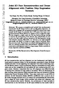
5.2. Performance Comparison for Different Subspaces For each testing face image, we also do 1 random initialization as above. The searching results are compared with the labelled shapes in the test data. We use point-topoint (Pt-Pt) error and point-to-boundary (Pt-Bd) error as the comparison measures. The point-to-point error is the average pixel distance from the found points on the search shape to the points of the labelled shape, and the point-toboundary error is the average pixel distance from the found points to the associated boundary on the labelled shape. The comparison results are shown in Table 2, where IO stands for independent optimization, GO stands for gradient descent optimization and PA stands for parallel analysis [18]. One typical searching example of AAM is given in Figure 2. We can see that the model with the explanations of 0.98 is too flexible so that it is easy to be stuck in local minimum(mouth and nose). However, the model with PA ex-

Figure 2. Result examples for AAM with different subspaces

6. Conclusion and Future Work In this paper, we proposed an unified subspace optimization method to solve the two separation problems with active statistical models: (1) the separation of the statistical model and the search process: these two parts are treated separately although they are closely correlated; (2) the separation of two kinds of parameters of the subspace: the number of components and the constraints. These two kinds of parameters are chosen separately although they both determine the subspace. This unified method is composed of two unification aspects: (1) unification of the statistical model and the search process: the subspace models are optimized according to the search procedure; (2) unification

of the number of components and the constraints: the two kinds of parameters are modelled in an unified way, such that they can be optimized jointly. The experimental results show that the proposed method is very promising. Future work includes applying this method to variations of ASM and AAM, and to other subspace-based algorithms.

References [1] S. Baker and I. Matthews. Equivalence and efficiency of image alignment algorithms. In Proceedings of IEEE Computer Society Conference on Computer Vision and Pattern Recognition, volume 1, pages 1090–1097, Hawaii, December 2001. [2] T. F. Cootes, G. J. Edwards, and C. J. Taylor. Active appearance models. In ECCV98, volume 2, pages 484–498, 1998. [3] T. F. Cootes and P. Kittipanya-ngam. Comparing variations on the active appearance model algorithm. In Proceedings of the British Machine Vision Conference, volume 2. [4] T. F. Cootes and C. J. Taylor. Constrained active appearance models. In Proceedings of IEEE International Conference on Computer Vision, pages 748–754, Vancouver, Canada, July 2001. [5] T. F. Cootes and C. J. Taylor. Statistical models of appearance for computer vision. Technical report, www.isbe.man.ac.uk/˜bim/refs.html, 2001. [6] T. F. Cootes, C. J. Taylor, D. H. Cooper, and J. Graham. Active shape models: Their training and application. CVGIP: Image Understanding, 61:38–59, 1995. [7] C. D. and C. T.F. A comparison of shape constrained facial feature detectors. In Proceedings of IEEE International Conference on Automatic Face and Gesture Recognition, pages 375–380, May 2004. [8] R. H. Davies, T. F. Cootes, and C. J. Taylor. A minimum description length approach to statistical shape modelling. IEEE Transactions on Medical Imaging, 21:525–537, 2002. [9] G. J. Edwards, T. F. Cootes, and C. J. Taylor. Interpreting face images using active appearance models. In Proc. International Conference on Automatic and Gesture Recognition, pages 300–305, Japan, 1998. [10] C. Goodall. Procrustes methods in the statistical analysis of shape. Journal of the Royal Statistical Society B, 53(2):285– 339, 1991. [11] A. Hill and C. J. Taylor. A framework for automatic landmark identification using a new method of nonrigid correspondence. IEEE Transactions on Pattern Analysis and Machine Intelligence, 22(3). [12] X. Hou, S. Li, and H. Zhang. Direct appearance models. In Proceedings of IEEE Computer Society Conference on Computer Vision and Pattern Recognition, number 1, pages 828–833, Hawaii, December 2001. [13] M. Kass, A. Witkin, and D. Terzopoulos. Snakes: Active contour models. In Proceedings of IEEE International Conference on Computer Vision, pages 259–268, 1987. [14] C. Liu, H.-Y. Shum, and C. Zhang. Hierarchical shape modeling for automatic face localization. In Proceedings of the

[15] [16]

[17]

[18]

[19]

[20]

[21]

[22]

[23]

[24]

European Conference on Computer Vision, number II, pages 687–703, Copenhagen, Denmark, May 2002. A. Martinez and R.Benavente. The AR face database. Technical Report 24, CVC, June 1998. P. J. Phillips, H. Moon, S. A. Rizvi, and P. J. Rauss. The FERET evaluation methodology for face-recognition algorithms. IEEE Transactions on Pattern Analysis and Machine Intelligence, 22(10):1090–1104, 2000. M. Rogers and J. Graham. Robust active shape model search. In Proceedings of the European Conference on Computer Vision, number IV, pages 517–530, Copenhagen, Denmark, May 2002. M. B. Stegmann, B. K. Ersboll, and R. Larsen. FAME a flexible appearance modeling environment. IEEE Transactions on Medical Imaging, 22(10):1319–1331, October 2003. B. van Ginneken, A. F. Frangi, J. J. Staal, B. M. ter Haar Romeny, and M. A. Viergever. Active shape model segmentation with optimal features. IEEE Transactions on Medical Imaging, 21(8):924–933, August 2002. L. Wiskott, J. Fellous, N. Kruger, and C. V. malsburg. Face recognition by elastic bunch graph matching. IEEE Transactions on Pattern Analysis and Machine Intelligence, 19(7):775–779, 1997. S. Yan, M. Li, H. Zhang, and Q. Cheng. Ranking prior likelihood distributions for bayesian shape localization framework. In Proceedings of IEEE International Conference on Computer Vision, volume 1, pages 51 – 58, Nice, France, October 2003. S. C. Yan, C. Liu, S. Z. Li, L. Zhu, H. J. Zhang, H. Shum, and Q. Cheng. Texture-constrained active shape models. In Proceedings of the First International Workshop on Generative-Model-Based Vision (with ECCV), Copenhagen, Denmark, May 2002. A. L. Yuille, D. Cohen, and P. W. Hallinan. Feature extraction from faces using deformable templates. In Proceedings of IEEE Computer Society Conference on Computer Vision and Pattern Recognition, pages 104–109, 1989. Y. Zhou, L. Gu, and H. Zhang. Bayesian tangent shape model: estimating shape and pose parameters via bayesian inference. In Proceedings of IEEE Computer Society Conference on Computer Vision and Pattern Recognition, volume 1, pages 109 – 116, Wisconsin, USA, June 2003.