Face Recognition and Pose Estimation with Parametric ... - CiteSeerX

Face Recognition and Pose Estimation with Parametric Linear Subspaces Kazunori Okada1 and Christoph von der Malsburg2,3 1

2

3

Department of Computer Science San Francisco State University San Francisco, CA 94132-4163 USA [email protected] Frankfurt Institute of Advanced Studies Science Campus Riedberg 60438 Frankfurt, Germany [email protected] Computer Science Department University of Southern California Los Angeles, CA90089-2520 USA

Summary. We present a general statistical framework for modeling and processing head pose information in 2D grayscale images: analyzing, synthesizing, and identifying facial images with arbitrary 3D head poses. The proposed framework offers a compact view-based data-driven model which provides bidirectional mappings between facial views and their corresponding parameters of 3D head angle. Such a mapping-based model implicitly captures 3D geometric nature of the problem without explicitly reconstructing a 3D structural model from data. The proposed model consists of a hierarchy of local linear models that cover a range of parameters by piecing together a set of localized models. This piecewise design allows us to accurately cover a wide parameter range, while the linear design, using efficient principal component analysis and singular value decomposition algorithms, facilitates generalizability to unfamiliar cases by avoiding overfitting. We apply the model to realize robust pose estimation using the view-to-pose mapping and pose-invariant face recognition using the proposed model to represent a known face. Quantitative experiments are conducted using a database of Cyberware-scanned 3D face models. The results demonstrate high accuracy for pose estimation and high recognition rate for previously unseen individuals and views for a wide range of 3D head rotation.

1 Introduction Face recognition is one of the most interesting and challenging problems in computer vision and pattern recognition. In the past many aspects of this problem have been rigorously investigated because of its importance for realizing various applications and understanding our cognitive processes. For

2

Kazunori Okada and Christoph von der Malsburg,

reviews, we refer the reader to [37, 6, 42]. Past studies in this field have revealed that our utmost challenge is to reliably recognize people in the presence of image/object variations that occur naturally in our daily life [32]. As head pose variation is one of the most common variations,it is an extremely important factor for many application scenarios. There have been a number of studies which specifically addressed the issue of pose invariance in face recognition [2, 31, 23, 20, 38, 3, 1, 13, 11, 16, 12, 15, 41, 30, 40, 5]. Despite the accumulation of studies and the relative maturity of the problem, however, performance of the state-of-the-art has unfortunately remained inferior to human ability and sub-optimal for practical use when there is no control over subjects and when one must deal with an unlimited range of full 3D pose variation. Our main goal is to develop a simple and generalizable framework which can be readily extended beyond the specific focus on head pose (e.g., illumination and expression), while improving the pose processing accuracy of the state-of-the-art. For this purpose, we propose a general statistical framework for compactly modeling and accurately processing head pose information in 2D images. The framework offers means for analyzing, synthesizing, and identifying facial images with arbitrary head pose. The model is data-driven in the sense that a set of labeled training samples are used to learn how facial views change as a function of head pose. For realizing the compactness, the model must be able to learn from only a few samples by generalizing to unseen head poses and individuals. Linearity is emphasized in our model design, which simplifies the learning process and facilitates generalization by avoiding typical pitfalls of non-linearity, such as overfitting [4]. For pose-insensitive face recognition, previous work can roughly be categorized into two types: single-view and multi-view approaches. Single-view approaches are based on person-independent transformation of test images [23, 20, 16]. Pose invariance is achieved by representing each known person by a facial image with a fixed canonical head pose and by transforming each test image to the canonical pose. This forces head pose of test and gallery entries to always be aligned when they are compared for identification. An advantage of this approach is the small size of the known-person gallery. However, recognition performance tends to be low due to the difficulty of constructing an accurate person-independent transformation. The multi-view approach [2, 3, 12, 41], on the other hand, is based on a gallery that consists of views of multiple poses for each known person. Pose-invariance is achieved by assuming that for each input face there exists a view with the same head pose as the input for each known person in the gallery. These studies have reported generally better recognition performance than the single-view approach. The large size of the gallery is, however, a disadvantage of this approach. The recognition performance and the gallery size have a trade-off relationship; better performance requires denser sampling of poses, increasing the gallery size. Larger gallery size makes it difficult to scale the recognition system to larger sets of known people and makes the recognition process more time-consuming.

Face Recognition and Pose Estimation with Parametric Linear Subspaces

3

One solution to the trade-off problem is to represent each known person by a compact model. Given the multi-view gallery, each set of views of a known person can be used as training samples to learn such a personalized model, reducing the gallery size while maintaining high recognition performance. The parametric eigenspace method of Murase and Nayar [25] and the virtual eigen-signature method of Graham and Allinson [13] are successful examples of this approach. These methods represent each known person by compact manifolds in the embedded subspace of the eigenspace. Despite their good recognition performance, generalization capability is their shortcoming. Both systems utilized non-linear methods (cubic-spline for the former and radial basis function network for the latter) for parameterizing/modeling the manifolds. Such methods have a tendency to overfit peculiarities in training samples, compromising capability to generalize over unseen head poses. The solution proposed here emphasizes linearity in model design, facilitating such generalization, as well as model compactness. Our investigation explores the model-based solution of pose estimation, pose animation, and pose-insensitive face recognition using parametric linear subspace models. As a basic component, we exploit local principal component mapping (LPCMAP) [27], which offers a compact view-based model with bidirectional mappings between face views and 3D head angles. A mapping from face to pose we call analysis mapping and that from pose to face /it synthesis mapping. Concatenation of the two mappings creates an analysis-synthesis chain for model matching. Availability of such mappings avoids the necessity of an exhaustive search in the parameter space. Its parametric nature also provides an intuitive interface that permits clear interpretation of image variations and enables the model to continuously cover the pose variation thereby improving accuracy of the previous systems. Such a mapping-based model implicitly captures the three-dimensional geometric nature of the problem without explicitly reconstructing 3D facial structure from data. The model is learned by using efficient principal component analysis (PCA) and singular value decomposition (SVD) algorithms resulting in a linear form of the functions. They are however only locally valid due to their linearity. Therefore this local model is further extended to mitigate this limitation. The parametric piecewise linear subspace (PPLS) model [29] extends the LPCMAP for covering a wider pose range by piecing together a set of LPCMAP models. Our multiple-PPLS model further extends the PPLS in the sense of generalization over different individuals [26]. The discrete local models are continuously interpolated, improving the structurally discrete methods such as the view-based eigenface by Pentland et al. [31]. These proposed models are successfully applied to solve pose estimation and animation by using analysis and synthesis mappings, respectively. A novel pose-insensitive face recognition framework is also proposed by exploiting the PPLS model to represent each known person. In our recognition framework, the model matching with the PPLS models provides a flexible pose alignment of model views and input faces with arbitrary head poses, making the recogni-

4


tion invariant against pose variation. As a pure head pose estimation application, the analysis mapping can also be made to generalize inter-personally by using the multiple-PPLS model that linearly combines a set of personalized PPLS models. The rest of this article is organized as follows. In Section 2, we give an overview of our framework and introduce some basic terminologies. Section 3 describes the LPCMAP and PPLS models in details. Section 4 shows how we can extend the PPLS model inter-personally. In Section 5, we empirically evaluate effectiveness of the proposed models. In Section 6, we conclude this article by summarizing our contributions and discussing future work.

2 Problem Overview and Definitions Our problem here is to learn a data-driven statistical model of how facial appearance changes as a function of corresponding head angles and to apply such learned models for building a face recognition system that is insensitive to pose variation. The following introduces formal descriptions of our problem, as well as terminology used throughout this paper. 2.1 Statistical Models of Pose Variation Analysis and Synthesis Mappings We employ the parametric linear subspace (PLS) model [27, 29] for representing pose-modulated statistics. A PLS model consists of bidirectional, continuous, multivariate, mapping functions between a vectorized facial image v and 3D head angles θ. We call a mapping AΩ from the image to angles analysis mapping, and its inverse SΩ synthesis mapping: Ω

AΩ : v −→ θ Ω

SΩ : θ −→ v(Ω),

(1)

where Ω denotes a model instance that is learned from a set of training samples. We suppose that a set of M training samples, denoted by M pairs {(vm , θ m )|m = 1, .., M }, is given where a single labeled training sample is denoted by a pair of vectors (vm , θ m ), vm being the m-th vectorized facial image, and θ m = (θm1 , θm2 , θm3 ) the corresponding 3D head angles of the face presented in vm . An application of the analysis mapping can be considered as pose estimation. Given an arbitrary facial image v ∈ / {v1 , .., vM }, AΩ provides a 3D head ˆ = AΩ (v) of a face in v. On the other hand, an application angle estimate θ of the synthesis mapping provides a means of pose transformation or facial animation. Given an arbitrary 3D head angle θ ∈ / {θ 1 , .., θ M }, SΩ provides a ˆ = SΩ (θ) whose head is rotated according synthesized sample or model view v to the given angle but its appearance is due to the learned model Ω.


5

Personalized and Interpersonalized Models The type of training samples used for learning a model determines the nature of a specific PLS model instance. A model is called personalized when it is learned with pose-varying samples from a single individual. In this case, both analysis and synthesis mappings become specific to the person presented in the training set. Therefore the synthesis mapping output v(Ω) exhibits personal appearance that solely depends on Ω encoding specificities of the person, while its head pose is given by an input to this mapping. On the other hand, a model is called interpersonalized when the training set contains multiple individuals. For pose estimation, this provides a more natural setting where the analysis mapping AΩ continuously covers not only head pose variations but also variations over different individuals. 2.2 Pose-Insensitive Face Recognition Model Matching Given an arbitrary person’s face as input, a learned PLS model can be fit against it by concatenating the analysis and synthesis mappings. We call this model matching process the analysis-synthesis chain (ASC) process: Ω

Ω

MΩ : v −→ θ −→ v(Ω).

(2)

The output of ASC is called the model view v(Ω). It provides a facial view v(Ω) of the person learned in Ω whose head pose is aligned to the input face in v. This process not only fits a learned model to the input but also gives simultaneously a 3D pose estimate as a byproduct that can be used for other application purposes. Note that, when matching a personalized PLS model to a different person’s face, the resulting model view can be erroneous due to the pose estimation errors caused by the identity mismatch. To overcome this problem, the AΩ of an interpersonalized model [26] can be exploited for reducing pose estimation errors. For the purpose of face recognition, however, these errors actually serve as an advantage because it makes model views of mismatched individuals less similar to the input helping to single out the correct face. Moreover such errors are typically small due to the geometrical proximity of different faces. Overview of the Proposed Recognition Framework Figure 1 illustrates our framework for pose-insensitive face recognition. The framework employs the PLS model as the representation of a known person. For each known person, a personalized model is learned from the pose-varying samples of the person. We call a database of P known people, as a set of learned personalized models {Ωp |p = 1, .., P }, the known-person gallery. Given

6

Kazunori Okada and Christoph von der Malsburg, Test Image

ANALYSIS Model 1

Model 2

Model 3

Model N

Known Person Gallery SYNTHESIS

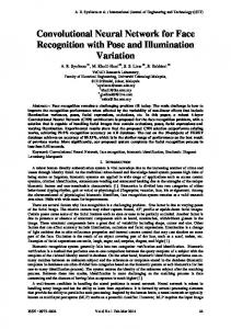
Nearest Neighbor Classification Fig. 1. Pose-insensitive face recognition framework with parametric linear subspace models used to represent each known person.

Model View Test Image

0.906 1 0.912

0.784 2 0.876

0.883 3 0.915

Best View

Fig. 2. An illustrative example of face recognition with pose variation using the model-based and the example-based systems.

a test image of an arbitrary person with an arbitrary head pose, each model in the gallery is matched against the image by using its ASC process. The process results in pose-aligned model views of all known persons. After this pose alignment, the test image is compared against the model views in nearest neighbor classification fashion. In this scheme, the view-based comparison only occurs between views of the same pose improving the recognition performance. Figure 2 illustrates the advantage of the proposed model-based method over an example-based multi-view method using a gallery of three known persons. A set of training samples for each person is used to construct the

Face Recognition and Pose Estimation with Parametric Linear Subspaces a

b

c

d

7

e

Input Views

Model Views

Best Views by MVS

Best View by SVS

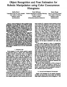
Fig. 3. Comparison of three recognition frameworks in terms of pose-alignment ability. Model views shown in the second row are given by the proposed method. MVS: example-based multi-view system; SVS: example-based single-view system. See texts for their description.

multi-view gallery entry. The top row displays model views of three learned models; the bottom row displays the best views of each known person that are most similar to the test image. Decimal numbers shown adjacent to the images denote their similarity to the test. There were no views in the gallery whose head pose was the same as the test image shown in the left. Therefore head pose of the test and the best matched views are always different. This results in a mis-identification by the multi-view system. On the other hand, the model-based solution, constructed by using the exactly same samples as in the multi-view system, identifies the test image correctly. This is realized by the model’s ability to generalize to unseen views, resulting in model views whose head pose is better aligned to the test. The proposed framework flexibly aligns head pose of the inputs and model views at an arbitrary pose, exploiting the PLS’s continuous generalization capability to unseen views. Figure 3 and Table 1 illustrate this advantage in comparison with two other recognition frameworks: the multi-view (MVS) and single-view (SVS) systems. Given facial images with arbitrary head poses shown in the first row, a PLS, learned for this face, can provide model views whose head pose is well aligned to the inputs. MVS provides the most similar view (best view) to the input among the training samples used to learn the model, while SVS employs always the same frontal view that acts as sole representation of the person. The figure shows that the proposed model appears to provide better pose-alignment than the two other systems. Table 1 shows actual facial similarity values between the inputs and the three different types of model or best view. The standard deviation shown in the right column

8

Kazunori Okada and Christoph von der Malsburg, Model Type a b c d e std.dev. Model Views 0.915 0.871 0.862 0.891 0.878 0.0184 Best Views by MVS 0.930 0.872 0.876 0.913 0.897 0.0220 Best View by SVS 0.926 0.852 0.816 0.878 0.862 0.0359

Table 1. Similarity scores between the test input and different types of model and best views in Figure 3.

indicates the degree of invariance against the pose variations by each framework. The parametric linear model provided the smallest standard deviation among the three, demonstrating the model’s favorable characteristics toward pose-insensitivity.

3 Parametric Linear Subspace Model This section describes two instances of the PLS model: the linear principal component-mapping (LPCMAP) model [27] and the parametric piecewise linear subspace (PPLS) model [29]. The PPLS model employs a set of LPCMAP models, each of which realizes continuous analysis and synthesis mappings. For maintaining the continuous nature in a global system, we consider that local mapping functions cover the whole parameter space, without imposing a rigid parameter window. Due to the linearity, however, the range over which each local mapping is accurate is limited. In order to cover a wide range of continuous pose variation, a PPLS model pieces together a number of local models distributed over the 3D angle space of head poses. In order to account for the local model’s parameter-range limitation, each model is paired with a radialbasis weight function. The PPLS then performs a weighted linear combination of the outputs of the local models, realizing a continuous global function. The following introduces details of these models. 3.1 Linear PCMAP Model The LPCMAP is a PLS model that realizes continuous, but only locally valid, bidirectional mapping functions. It consists of a combination of two linear systems: 1) linear subspaces spanned by principal components (PCs) of training samples and 2) linear transfer matrices, which associate projection coefficients of training samples onto the subspaces and their corresponding 3D head angles. It linearly approximates the entire parameter space of head poses by a single model. Shape-Texture Decomposition and Image Reconstruction The LPCMAP model treats shape and texture information separately in order to utilize them for different purposes. It has also been shown in the literature


9

Training Sample

20 Landmarks Found

20

Locations of the Landmarks

Local Gray-Level Distribution Captured in 20 Jets

40 80 node1 node2 node3

node20

Shape Representation A Single 40-Component Vector

Jet1 Jet2 Jet3

Jet20

Texture Representation 20 80-Component Vectors

Fig. 4. Shape and texture decomposition process, illustrating parameter settings used for our experiments in Section 5. The number of landmarks N = 20 and the length of a texture vector L = 80 with a bank of 5-level and 8-orientation 2D complex Gabor filters.

that combining shape with shape-free texture information improves recognition performance [38, 7, 21]. Figure 4 illustrates the process of decomposing shape and texture information in facial images. First, N predefined landmarks are located in each facial image vm by a landmark finder or other means. Using this location information, shape and texture representations (xm , {jm,n }) are extracted from the image. The shape is represented by an array xm ∈ R2N of object-centered 2D coordinates of the N landmarks. Texture information, on the other hand, is represented by a set of spatially sparse local feature vectors sampled at the N landmark points. A multi-orientation and multiscale Gabor wavelet transformation [8] is used to define local features. The texture representation {jm,n ∈ RL |n = 1, .., N } stands for a set of Gabor jets (L-component complex coefficient vector of the Gabor transform) sampled at the N landmarks [19, 39, 28]. Let Dx and Dj denote operations of the shape and texture decomposition, respectively: xm = Dx (vm ) jm,1 , .., jm,N = Dj (vm ).

(3)

As an inverse operation, a gray-level facial image can be reconstructed approximately from a pair of shape and texture representations (xm , {jm,n }), following the work by Poetzsch et al. [33]. R denotes this reconstruction operation: vm = R(xm , jm,1 , .., jm,N ). (4)


10

Training Samples

e1

v

≅

E( v)

( w1 * + ( w2 * + + + ( wp *

)

SP

e2

Shape

) Shape Reps.

Pose PS

Texture Reps.

PCA

PCA

ST

ep

)

Shape Model GLOBAL

(a)

Texture Model LOCAL (For N-Landmarks)

(b)

Texture

(c)

Fig. 5. Learning processes of the LPCMAP model: (a) PCA subspace model by Sirovich and Kirby [36], (b) shape and texture models using linear subspaces, and (c) linear transfer matrices relating different model parameters A rectangle in (b) denotes a set of training samples and an ellipse denotes a PCA subspace model.

Learning Linear Subspace Models As the first step of the model learning process, we extract a small number of significant statistical modes from facial training images using Principal Component Analysis (PCA), as illustrated in Figure 5. Given training samples {(vm , θ m )|m = 1, .., M }, a set of extracted shape representations {xm } is subjected to PCA [34], solving the eigen decomposition problem of the centered sample covariance matrix, XX t yp = λp yp , where X is a 2N M column sample matrix. This results in an ordered set of 2N principal components (PCs) {yp |p = 1, .., 2N } of the shape ensemble. We call such PCs shape PCs. The local texture set {jm,n } at a landmark n is also subjected to PCA, resulting in an ordered set of L PCs {bs,n |s = 1, .., L}. We cal such PCs texture PCs. Performing this procedure for all the N landmarks results in a set of local texture PCs {bs,n |s = 1, .., L; n = 1, .., N }. The subspace model [36, 31] is defined by a vector space spanned by a subset of the PCs in decreasing order of their corresponding variances as illustrated in Figure 5(a). An image v is approximated as the sum of the average image E(v) and the PCs (e1 , .., ep ). The weight vector (w1 , .., wp ) is defined by orthogonal projection onto the subspace and serves as a compact representation of the image v. Due to the orthonormality of PCs, a linear combination of the PCs with the above mixing weights provides the best approximation of an original representation which minimizes the L2 reconstruction error. As illustrated in Figure 5(b), a shape model Y is constructed by the first P0 ≤ 2N shape PCs, Y = (y1 , .., yP0 )t . And a texture model {Bn } is then constructed by the first S0 ≤ L texture PCs at each landmark n, {Bn = (b1,n , .., bS0 ,n )t |n = 1, .., N }. These subspace models are used to parameterize and compress a centered input representation by orthogonally projecting it onto the subspace:


qm = Y (xm − ux ) ux =

M 1 X xm M m=1

rm,n = Bn (jm,n − ujn ) ujn =

M 1 X jm,n . M m=1

11

(5)

(6)

We call the projection coefficient vectors for shape representation qm ∈ RP0 shape parameters and those of texture representation rm,n ∈ RS0 texture parameters, respectively. We also refer to these parameters (equivalent to the weight vector in Figure 5(a)) as model parameters collectively. xm ≈ ux + Y t qm

(7)

jm,n ≈ ujn + (Bn )t rm,n

(8)

Learning Linear Transfer Matrices As the second step of the learning process, model parameters are linearly associated with head pose parameters for realizing direct mappings between v and θ, as illustrated in Figure 5(c). Clearly, the model parameters are non-linearly related to the 3D head angles, and therefore the intrinsic mapping between them is non-linear. In order to linearly approximate such non-linear mapping, we first transform the 3D head angles θ m = (θm,1 , θm,2 , θm,3 ) to pose parameters ϕm ∈ RT ≥3 such that the mapping between the pose and model parameters can be linearly approximated. We consider the following trigonometric function K for this purpose. ϕm = K(θ m ) = (cos (θ˜m,1 ), sin (θ˜m,1 ), cos (θ˜m,2 ), sin (θ˜m,2 ), cos (θ˜m,3 ), sin (θ˜m,3 )) PM 1 θ˜m,i = θm,i − uθi uθ = (uθ1 , uθ2 , uθ3 ) = M m=1 θ m (9) There exists an inverse transformation K−1 such that ϕm,2 ϕm,4 ϕm,6 θ m = K−1 (ϕm ) = uθ + (arctan( ), arctan( ), arctan( )) (10) ϕm,1 ϕm,3 ϕm,5 For both the analysis and synthesis mappings, the pose parameters ϕm are linearly related only with the shape parameters qm . ϕm = F qm

(11)

qm = Gϕm

(12)

A T ×P0 transfer matrix F (denoted as SP in Figure 5(c)) is learned by solving an overcomplete set of linear equations, F Q = Φ, Q = (q1 , .., qM ), Φ = (ϕ1 , .., ϕM ). The Singular Value Decomposition (SVD) [34] is used to solve this linear system. Moreover, a P0 × T transfer matrix G (denoted as PS in

12


Figure 5(c)) is also learned by solving, GΦ = Q, in the same manner. For the synthesis mapping, the shape parameters qm are linearly related with the texture parameters rm,n at each landmark n. {rm,n = Hn qm |n = 1, .., N }

(13)

A set of S0 × P0 transfer matrices {Hn } (denoted as ST in Figure 5(c)) is learned by solving, Hn Q = Rn , Rn = (r1,n , .., rM,n ), by using SVD for all the N landmarks. Model Definition The above two learning steps generate a set of data entities that collectively capture facial appearance in a given set of training samples. A LPCMAP model LM is defined by such data entities that are learned from training samples LM := {ux , {ujn }, uθ , Y, {Bn }, F, G, {Hn }}, (14) where ux and {ujn } are average shape and texture representations, uθ is an average 3D head angle vector, Y and {Bn } are shape and texture models, F and G and {Hn } are shape-to-pose, pose-to-shape, and shape-to-texture transfer matrices. Mapping and Chain Functions The analysis and synthesis mappings are constructed as a function of the learned LPCMAP model LM , as illustrated in Figure 6. The analysis mapping function ALM (v) is given by combining formulae (3), (5), (11), and (10): ˆ = ALM (v) = uθ + K−1 (F · Y · (Dx (v) − ux )). θ

(15)

The analysis function only utilizes the shape information of faces, following results of our preliminary experiments in which the head angles are better correlated with the shape representations than the texture representations [26]). The synthesis mapping function S(θ) is given by relating the 3D head angles to the shape coefficients and the shape coefficients to the texture coefficients. Because we have separate shape and texture decompositions, we address distinct synthesis processes for shape and texture. We refer to the shape and texture synthesis mapping functions as SS and T S, respectively. The shape synthesis mapping function SS LM (θ) is given by combining formulae (9), (12), and (7), using only the shape information similar to the analysis function. On the other hand, the texture synthesis mapping function T S LM (θ) is given by formulae (9), (12), (13), and (8), utilizing the correlation between shape and texture parameters. The synthesis mapping function SLM (θ) is then given by substituting the shape and texture synthesis functions to formula (4):


13

Input Image

Analysis (Pose Estimation) Output

( α, β, γ )

Head arctan Pose Angles Parameters

SP

Landmark Finding Shape Rep. Orthographic Projection Shape Model Parameters

ASC: Analysis-Synthesis Chain ( α, β, γ )

Head Angles Input

Pose TFT Parameters

PS

Shape Model ST Texture Model Parameters Parameters Linear Combination Shape Rep.

Synthesis (Pose Transformation)

Texture Rep.

Image Reconstruction Synthesized Image

Fig. 6. Analysis and synthesis mapping and analysis-thesis-chain functions. Trigonometric transfer functions K and K−1 are denoted by TFT and arctan, respectively. SP, PS and ST denote the transfer matrices shown in Figure 5(c).

ˆ = SLM (θ) = R(SS LM (θ), T S LM (θ)) v ˆ = SS LM (θ) = ux + Y t · G · K(θ − uθ ) x {jˆn |n = 1, .., N } = T S LM (θ) = {ujn + Bn · Hn · G · K(θ − uθ )|n = 1, .., N }. (16) Finally, the ASC function M(v) is given by concatenating Eq. (15) and Eq. (16) as shown in Figure 6: ˆ = MLM (v) = R(SS LM (ALM (v)), T S LM (ALM (v))). v

(17)

3.2 Parametric Piecewise Linear Subspace Model Model Definition The parametric piecewise linear subspace (PPLS) model [29] extends the LPCMAP model by using the piecewise linear approach [35]. Due to the linear approximation, the LPCMAP model can only be accurate within a limited range of pose parameters. A piecewise linear approach approximates the nonlinear pose variation within a wider range by piecing together a number of locally valid models distributed over the pose parameter space. The PPLS model P M consists of a set of K local models in the form of the abovedescribed LPCMAP model:

14


Input Sample

pose estimation by the PPLS system

Z 0.002

Y

3D Angle Space 0.498

0

X 0.3

0

PPLS Synthesized Sample

0.19

0.002

synthesized model views by the local models

Weighted Averaging

7 local model centers 3D pose of the test sample (14, 24, 0) Fig. 7. A sketch of the PPLS model with seven LPCMAP models. An input image is shown at the top-left. Model centers of the LPCMAPs are denoted by circles. Pose estimation is performed by applying the analysis mapping AP M , giving the global estimate denoted by a filled circle. Pose transformation, on the other hand, is performed by applying the synthesis mapping SP M . Model views, shown next to the model centers, are linearly combined with Gaussian weights, resulting in the global synthesis shown at the bottom-left.

P M := {LMk |k = 1, .., K}.

(18)

We assume that the local models are learned by training data sampled from appropriately distanced local regions of the 3D angle space: the 3D finite parameter space spanned by the head angles. Each set of the local training k samples is associated with a model center, the average 3D head angles uLM , θ which specifies the learned model’s location in the 3D angle space. Figure 7 illustrates seven local models distributed in the 3D angle space. Model centers are denoted by circles and model views of the input are also shown next to them. Missing components of shape representations due to large head rotations are handled by the mean-imputation method [22], which fills in each missing component by a mean computed from all available data at the component dimension. Mapping and Chain Functions The analysis mapping function AP M of the PPLS model is given by averaging K local pose estimates with appropriate weights as illustrated in Figure 7: ˆ = AP M (v) = θ

K X k=1

wk ALMk (v).

(19)


15

Similarly, the synthesis mapping function SP M is given by averaging K locally synthesized shape and texture estimates with the same weights as illustrated in Figure 7: ˆ = SP M (θ) = R(SS P M (θ), T S P M (θ)) v P ˆ = SS P M (θ) = K x (20) k=1 wk SS LMk (θ) P K {jˆn } = T S P M (θ) = k=1 wk T S LMk (θ). A vector of the weights w = (w1 , .., wK ) in Eq. (19) and Eq. (20) is responsible for localizing the output space of the LPCMAP models, since their outputs themselves are continuous and unbounded. For this purpose, we defined the weights, as a function of the input pose, by using a normalized Gaussian function of distance between an input pose and each model center LMk )

ρ (θ−uθ wk (θ) = PK k

LM ρk (θ−uθ k ) k=1

ρk (θ) =

√ 1 2πσk

2

exp(− kθk ) 2σ 2 k

(21)

where σk denotes the k-th Gaussian width. It is set by the standard deviation of the 3D head angle vectors used for learning LMk and determines the ˆ and v ˆ . The weight extent to which each local model influences the outputs θ value reaches maximum when the input pose coincides with one of the model centers; it decays as the distance increases. Outputs of local models that are located far from an input pose can become distorted because of the pose range limitation. However, these distorted local outputs do not strongly influence the global output because their contribution is suppressed by relatively low weight values. The ASC function M(v) is again given by connecting an analysis output to a synthesis input. ˆ = MP M (v) = R(SS P M (AP M (v)), T S P M (AP M (v))) v

(22)

Gradient Descend-based Pose Estimation Note that Eq. (19) cannot be solved in closed-form because its r.h.s. include the weights as a function of an unknown θ. To overcome this problem, a gradient descent-based iterative solution is formulated. Let a shape vector x be an input to the algorithm. Also let xi and θ i denote the shape and angle estimates at the i-th iteration. The algorithm iterates the following formulae until the mean-square error k∆xi k2 becomes sufficiently small: ∆x = x − xi , PK i 0 k=1 wk (θ i )ALMk (∆xi ), θ = θ i + η∆θ i , PKi+1 = k=1 wk (θ i+1 )SS LMk (θ i+1 ),

∆θ i = xi+1

(23)

where η is a learning rate and A0 is a slight modification of Eq. (15) that replaces a vectorized facial image v by a shape (difference) vector ∆xi . The

16


initial conditions x0 and θ 0 are given by the local model whose center shape k uLM is most similar to x. x Note that the weighted sum of the analysis mappings in (23) is used as an approximation of the gradient of θ with respect to x at the current shape estimate xi . In the PPLS model, such gradients are only available at the K discrete model centers. The second formula in (23), therefore, interpolates the K local gradient matrices for computing the gradients at an arbitrary point in the 3D angle space. The good local accuracy of the LPCMAP model shown in [27] supports the validity of this approximation. When a sufficient number of local models are allocated in the 3D angle space, the chance of being trapped at a local minimum should decrease. In our experimental setting described in the next section, the above initial condition settings resulted in no local minimum trappings significantly away from the global minimum. Note also that the algorithm performs pose estimation and shape synthesis simultaneously since it iterates between pose and shape in each loop. This gives an alternative for the shape synthesis, although the global synthesis mapping in (20) remains valid.

4 Interpersonalized Pose Estimation As mentioned in Section 2.1, a single system should be able to solve the pose estimation task across different individuals by exploiting the geometrical similarity between faces. In the previous sections, we focused on how to model pose variations by using an example of personalized PLS models. This section discusses how to extend the PLS framework to capture variations due to head pose and individual differences simultaneously. The resulting interpersonalized model is applied to realize pose estimation across different people. There are two approaches for realizing such an interpersonalized PLS model. The first is simply to train a LPCMAP or PPLS model by using a set of training samples that contain different-pose views from multiple people. The generic design of the proposed PLS models allows this straightforward extension, we must, however, empirically validate if the learned linear model adequately captures both variations correctly. After learning, both LM and P M can be used in the manner described in Section 3 for exploiting the corresponding analysis-synthesis mappings and ASC model matching. We refer to this type of model as single-PLS model. The second approach is to linearly combine a set of personalized models similar to the way we constructed PPLS using a set of LPCMAPs. We refer to this type of model as multiple-PPLS model. A multiple-PPLS model M M consists of a set of P personalized models in the form of PPLS: M M := {P Mp |p = 1, .., P }.

(24)

We assume that each individual PPLS model is personalized by learning it with pose-varying samples of a specific person and that the training samples


17

cover an adequate range of head poses in the 3D angle space. The analysis mapping function AM M of the multiple-PPLS model is then defined by a weighted linear combination of P pose estimates by the personalized models, realizing an interpersonalized pose estimation: ˆ = AM M (v) = θ

P X

wp AP Mp (v).

(25)

p=1

The weight vector w = (w1 , .., wP ) is responsible for choosing appropriate personalized models and ignoring models that encode faces very different from the input. We consider an error of shape reconstruction errp (x) by using a shape-only analysis-synthesis chain of the PPLS model p. In a way similar to (21) we then let a normalized Gaussian function of such errors indicate fidelity of the personalized models to the input: ρ (errp (x)) wp (θ) = PP p p=1

ρp (errp (x))

errp (x) = x − xˆp = x − SS P Mp (AP Mp (x)) kerrp (x)k2 1 ρp (θ) = √2πσ exp(− 2σ ), 2 p

(26)

p

where a shape synthesis mapping SS P Mp of the multiple-PPLS model is defined similar to (25) and σp denotes the Gaussian width of model p.

5 Experiments 5.1 Data Set For evaluating our system’s performance we must collect a large number of samples with controlled head poses, which is not an easy task. For mitigating this difficulty, we use 3D face models pre-recorded by a Cyberware scanner. Given such data, relatively faithful image samples with an arbitrary, but precise, head pose can easily be created by image rendering. We used 20 heads randomly picked from the ATR-Database [17], as shown in Figure 8. For each head, we created 2821 training samples. They consist of 7 local sample sets each of which covers a pose range of ±15 degrees at one-degree intervals. These local sets are distributed over the 3D angle space such that they collectively cover a pose range of ±55 degrees along each axis of 3D rotations; their model centers are distanced by ±40 degrees from the frontal pose (origin of the angle space). We also created 804 test samples for each head. In order to test the model’s generalization capability to unknown head poses, we prepared test samples whose head poses were not included in the training samples. Head angles of some test samples were in between the multiple local models and beyond their ±15 degree range. They cover a pose range of ±50 degrees. For more details of the data, see our previous reports [26, 29].

18


Fig. 8. 20 frontal views rendered from the 3D face models.

For each sample, the 2D locations of 20 inner facial landmarks, such as eyes, nose and mouth, are derived by rotating the 3D landmark coordinates, initialized manually, and by projecting them onto the image plane. The explicit rotation angles of the heads also provide 3D head angles of the samples. The rendering system provides the self-occlusion information. Up to 10% of the total landmarks were self-occluded for each head. 5.2 Personalized Pose Estimation and View Synthesis We compare the PPLS and LPCMAP models learned using the training samples described above. The PPLS model consists of 7 local linear models, each of which is learned from one of the local training sets. On the other hand, a single LPCMAP model was learned from the total set of 2821 samples. The shape and texture representation are extracted using the specification N = 20 and L = 80 described in Figure 4. The PPLS model uses σk set to the sample standard deviation, gradient descent is done over 500 iterations, and η is set to 0.01. The learned models are tested with both 2821 training samples themselves and 804 separate test samples of unknown pose. We refer to the former by accuracy test and the latter by generalization test. Figure 9(a) compares average pose estimation errors of the PPLS and LPCMAP models in both accuracy and generalization tests. In the accuracy test, the average angular error with the first 8 PCs was 0.8 ± 0.6 and 3.0 ± 2.4 degrees and the worst error was 5.6 and 18.9 degrees for the PPLS and LPCMAP models, respectively. In the generalization test, the average error was 0.9±0.6 and 2.4±1.4 degrees, and the worst error was 4.5 and 10.2 degrees for the two models. Figure 9(b) compares average shape synthesis errors of the

Face Recognition and Pose Estimation with Parametric Linear Subspaces 5

5 PPLS LPCMAP

3.5 3 2.5 2 1.5 1 0.5 10

15 20 25 Number of Shape PCs

30

2 1.5

35

0 0

40

PPLS LPCMAP Average Position Error (pixels)

3.5 3 2.5 2 1.5 1 0.5

10


30

35

10


(a)

30

35

40

0.92 0.9 0.88

0.84 0

40

10

20

30 40 50 60 Number of Texture PCs

70

80

1

PPLS LPCMAP

PPLS LPCMAP

0.98

4 3.5 3 2.5 2 1.5

0.96 0.94 0.92 0.9 0.88

1 0.86

0.5 5

0.94

0.86

5

4.5

4

0.96

1

5

4.5 Average Angular Error (degrees)

3 2.5

0.5 5

5

0 0

3.5

Average Jet Similarity

0 0

PPLS LPCMAP

0.98

4 Average Jet Similarity

4

1

PPLS LPCMAP

4.5 Average Position Error (pixels)

Average Angular Error (degrees)

4.5

19

0 0

5

10


30

35

40

0.84 0

10

(b)

20

30 40 50 60 Number of Texture PCs

70

80

(c)

Fig. 9. Comparison of the PPLS and LPCMAP models in terms of pose estimation and transformation errors. The first and second rows show results of the accuracy and generalization tests, respectively. Errors (similarities) are plotted over the number of PCs used to construct a subspace. (a) pose estimation errors in degrees averaged over 3 rotation angles. (b) shape synthesis errors in pixels averaged over 20 landmarks. (c) texture synthesis error by Gabor jet similarity averaged over 20 landmarks.

two models in the two test cases. In the accuracy test, the average landmark position error with the first 8 PCs was 0.8 ± 0.4 and 2.2 ± 1.2 pixels, and the worst error was 3.0 and 7.6 pixels for the PPLS and LPCMAP models, respectively. In the generalization test, the average error was 0.9 ± 0.4 and 2.4 ± 0.7 pixels, and the worst error was 2.7 and 5.6 pixels for the two models. Figure 9(c) compares average similarities between synthesized texture vector ˆj and ground-truth texture vector j for the two models in the two test cases. Local texture similarity is computed as a normalized dot-product (cosine) of Gabor jet magnitudes, JetSim :=

amp(j)·amp(ˆj) , kamp(j)k kamp(ˆj)k

where amp extracts

magnitudes of a Gabor jet in polar coordinates and k · k denotes L2 vector norm. The similarity values range from 0 to 1, where 1 denotes equality of two jets. In the accuracy test, the average similarity with the first 20 texture PCs was 0.955 ± 0.03 and 0.91 ± 0.04, and the worst similarity was 0.81 and 0.73 for the PPLS and LPCMAP models, respectively. In the generalization test, the average similarity was 0.945 ± 0.03 and 0.88 ± 0.03, and the worst similarity was 0.82 and 0.77 for the two models. For all three tasks, the PPLS model greatly improved performance over the LPCMAP model in both test cases, resulting in sub-degree and sub-pixel accuracy. The results also show that the average errors between the two test cases were similar, indicating good generalization to unknown poses. As a reference for our texture similarity analysis, we computed average texture similarities

20


(a)

(b)

PPLS

TEST

LPCMAP

(c)

Fig. 10. Examples of synthesized model views by the PPLS model. In (a) and (b), model views in the first and second rows are reconstructed from ground-truth and synthesized pose-aligned samples, respectively. (a): training samples with known head pose (accuracy test case); (b): test samples with unknown head poses (generalization test case); (c): illustrative comparison of model views synthesized by the PPLS and LPCMAP models.

over 450 people from the FERET database [32]. The average similarity was 0.94 ± 0.03 for the same person pairs and 0.86 ± 0.02 for the most similar, but different, person pairs. The average similarity of the PPLS model was higher than that of the large FERET database, which validates the results of our texture similarity analysis. Figure 10 illustrates model views: images reconstructed from samples synthesized by formula (20) of the PPLS model. Note that facial images reconstructed by the P¨otzsch algorithm [33] do not retain original picture quality. This is because a transformation Dj from images to the Gabor jet representations is lossy due to coarse sampling in both the spatial and frequency domains. Nonetheless, these images still capture characteristics of faces fairly well. Figure 10(a) compares reconstructed images of original and synthesized


21

Test Samples Identification Compression SVS 59.9±10.6% 0.035% LPCMAP 91.6±5.0% 0.74% PPLS 98.7±1.0% 5% MVS 99.9±0.2% — Table 2. Average correct-identification and relative compression rates for four different systems.

training samples. The left-most column shows frontal views while the rest of columns show views with ±45 degree rotation along one axis. Figure 10(b) compares original and synthesized test samples. For all three cases, the original and synthesized model views were very similar, indicating good accuracy and successful generalization to unknown head poses. Figure 10(c) compares model views synthesized by the PPLS and LPCMAP models. The PPLS’s model view was more similar to the original than the LPCMAP’s model view. This agrees with the results of our error and similarity analyses. 5.3 Pose-Insensitive Face Recognition For comparison, we constructed four recognition systems with 20 known persons: 1) the single-view system (SVS), which represents each known person by a single frontal view, 2) the LPCMAP system with a gallery of LPCMAP models, 3) the PPLS system with a gallery of PPLS models, and 4) the multiview system (MVS), which represents each person by various raw views of the person. The LPCMAP, PPLS and MVS are constructed by using the same 2821 training samples per person; the SVS serves as a base-line. For both models, P0 and S0 are set to 8 and 20, respectively. The PPLS models consist of 7 local models and perform 500 iterations with η set to 0.01 for each test sample. Each pair of views is compared by an average of normalized dot-product similarities between the corresponding Gabor jet’s magnitudes. Table 2 summarizes the results of our recognition experiments. Identification rates in the table are averaged over the 20 persons; the compression rates represent the size of the known-person gallery as a fraction of the MVS. The results show that recognition performance of the PPLS system was more robust than the LPCMAP system (7% higher rate). Performance of our modelbased systems was much better than the base-line SVS. Identification rates of the PPLS and MVS were almost the same while the former compressed the data by a factor of 20. In some application scenarios, head pose information can be independently measured by the other means prior to identification. In such a case, the proposed recognition system can be realized by using only the synthesis mapping instead of model matching. Table 3 compares average identification rates of the two cases: with and without the knowledge of head pose. The results


22

PPLS LPCMAP Unknown: M(v) 98.7±1.0% 91.6±5.0% Known: S(θ) 99.3±0.7% 92.4±4.0% Table 3. Identification rates when head pose of tests is unknown or given as groundtruth. 5

5 Single−PPLS Multiple−PPLS(SIG=7) Multiple−PPLS(SIG=1) Baseline

4

4

3.5

3.5

3

2.5

2

1.5

3

2.5

2

1.5

1

1

0.5

0.5

0

0

5

10


30

35

Single−PPLS Multiple−PPLS(SIG=7) Baseline

4.5

Average Angluar Error (degrees)

Average Angluar Error (degrees)

4.5

40

0

0

Interpolation Test

5

10


30

35

40

Extrapolation Test

Fig. 11. Comparison of the single-PPLS and multiple-PPLS models for the interpolation and extrapolation tests in terms of interpersonalized pose estimation errors. Baseline plots indicate average pose estimation errors by the personalized models shown in Figure 9 for reference.

show that the knowledge of head pose gave a slight increase in recognition performance, however the increase was minimal. 5.4 Interpersonalized Pose Estimation For comparison, we tested both single-PPLS and multiple-PPLS models for two test cases: interpolation and extrapolation tests, using the data described in Section 5.1. For the interpolation (known persons) test, both models are trained with all the 56420 training samples (20 people × 2821 samples). A single-PPLS model with 7 LPCMAPs is trained with all the samples. On the other hand, a multiple-PPLS model is build by training each personalized model with 2821 samples for a specific person. These two models are then tested with the same 16080 test samples from the 20 individuals. For the extrapolation (unknown persons) test, each model is trained with 53599 training samples of 19 individuals, excluding training samples referring to the person being tested, so that the model does not contain knowledge of testing faces. The two models are trained in the same way as the interpolation test and tested with the same 16080 test samples. The same parameter settings of LPCMAP and PPLS models are used as described in Section 5.2.


23

Figure 11 compares the single-PPLS model and multiple-PPLS model in the two test settings. Down-triangles denote the average angular errors of the single-PPLS model and up-triangles denote those of the multiple-PPLS model with σp = 7 for all p. As reference, average pose estimation errors of the personalized model shown in Figure 9 are also included and denoted by solid lines without markers. Errors are plotted against 6 different sizes of the shape model. Our pilot study indicated that σp = 7 for all p is optimal for both interpolation and extrapolation cases. However σp = 1 for all p was optimal when only an interpolation test was considered. For this reason, errors with σp = 1 is also included for the interpolation test. When σp is set optimally for both test cases, the average errors of the two models were very similar between two test cases. With the first 8 shape PCs, the errors of the two models were the same: 2.0 and 2.3 degrees for the interpolation and extrapolation tests, respectively. For the interpolation test, the standard deviation of the errors and the worst error were 0.9 and 5.5 degrees for the single-PPLS model and 0.8 and 5.1 degrees for the multiplePPLS model. For the extrapolation test, the standard deviation and the worst error were 0.9 and 5.9 degrees for the former and 0.9 and 5.5 degrees for the latter. For both tests, the average errors of the two models are roughly 1 to 1.5 degrees larger than the baseline errors. When σp is set optimally for the interpolation condition, the multiple-PPLS model clearly outperformed the single-PPLS model, improving the average errors by roughly 1 degree and becoming similar to the baseline result (only 0.2 degree difference). These experimental results indicate that both models are fairly accurate, indicating the feasibility of the proposed approach to generalize over different persons.

6 Conclusion This article presents a general statistical framework for modeling and processing head pose information in 2D grayscale images: analyzing, synthesizing, and identifying facial images with arbitrary 3D head poses. Three types of PLS model are introduced. The LPCMAP model offers a compact viewbased model with bidirectional analysis and synthesis mapping functions. A learned model can be matched against an arbitrary input by using an analysissynthesis chain function that concatenates the two. The PPLS model extends the LPCMAP for covering a wider pose range by combining a set of local models. Similarly the multiple-PPLS model extends the PPLS for generalizing over different people by linearly combining a set of PPLSs. A novel pose-insensitive face recognition framework is proposed by using the PPLS model to represent each known person. Our experimental results for 20 people covering a 3D rotation range as wide as ±50 degree demonstrated the proposed model’s accuracy for solving pose estimation and pose animation tasks and robustness for generalizing to unseen head poses and individuals while compressing the data by a factor of 20 and more.

24


The proposed framework was evaluated by using accurate landmark locations and corresponding head angles computed by rotating 3D models explicitly. In reality, a stand-alone vision application based on this work will require a landmark detection system as a pre-process. A Gabor jet-based landmark tracking system [24] can be used to provide accurate landmark positions. It requires, however, the landmarks to be initialized by some other method. Pose-specific graph matching [18] provides an another solution but with much lower precision. In general, the landmark locations and head angles will contain measurement errors. Although our previous studies indicated robustness to such errors [26], more systematic investigation on this matter should be performed in future. Our future goal must address other types of variation such as illuminations and expressions for realizing more robust systems. There has been progress with variation of both illumination [9, 12] and expression [10, 14]. However, the issue of combining these variation-specific solutions into a unified system robust against the different types of variation simultaneously has not fully been investigated. Our simple and general design approach may help to reach this goal.

Acknowledgments The authors thank Shigeru Akamatsu and Katsunori Isono for making their 3D face database available for this study. This study was partially supported by ONR grant N00014-98-1-0242, by a grant by Google, Inc. and by the Hertie Foundation.

References 1. M. S. Bartlett and T. J. Sejnowski. Viewpoint invariant face recognition using independent component analysis and attractor networks. In Neural Information Processing Systems: Natural and Synthetic, volume 9, pages 817–823. MIT Press, 1997. 2. D. Beymer. Face recognition under varying pose. Technical Report A.I. Memo, No. 1461, Artificial Intelligence Laboratory, M.I.T., 1993. 3. D. Beymer and T. Poggio. Face recognition from one example view. Technical Report 1536, Artificial Intelligence Laboratory, M.I.T., 1995. 4. C. M. Bishop. Neural Networks for Pattern Recognition. Oxford University Press, New York, 1995. 5. X. Chai, L. Qing, S. Shan, X. Chen, and W. Gao. Pose invariant face recognition under arbitrary illumination based on 3d face reconstruction. In Proc. AVBPA, pages 956–965, 2005. 6. R. Chellappa, C. L. Wilson, and S. Sirohey. Human and machine recognition of faces: A survey. Proceedings of the IEEE, 83(5):705–740, 1995.


25

7. I. Craw, N. Costen, T. Kato, G. Robertson, and S. Akamatsu. Automatic face recognition: Combining configuration and texture. In Proc. Int. Conf. Automatic Face and Gesture Recognition, pages 53–58, Zurich, 1995. 8. J. G. Daugman. Complete discrete 2-D Gabor transforms by neural networks for image analysis and compression. IEEE Trans. Acoustics, Speech, and Signal Processing, 36:1169–1179, 1988. 9. P. Debevec, T. Hawkins, H. P. Tchou, C. Duiker, W. Sarokin, and M. Sagar. Acquiring the reflectance field of a human face. In Proceedings of Siggraph, pages 145–156, 2000. 10. G. Donato, M. S. Bartlett, J. C. Hager, P. Ekman, and T. J. Sejnowski. Classifying facial actions. IEEE Trans. Pattern Analysis and Machine Intelligence, 21(10):974–988, 1999. 11. S. Duvdevani-Bar, S. Edelman, A. J. Howell, and H. Buxton. A similarity-based method for the generalization of face recognition over pose and expression. In Proc. Int. Conf. Automatic Face and Gesture Recognition, pages 118–123, Nara, 1998. 12. A. S. Georghiades, P. N. Belhumeur, and D. J. Kriegman. From few to many: Generative models for recognition under variable pose and illumination. In Proc. Int. Conf. Automatic Face and Gesture Recognition, pages 277–284, Grenoble, 2000. 13. D. B. Graham and N. M. Allinson. Characterizing virtual eigensignatures for general purpose face recognition. In Face Recognition: From Theory to Applications, pages 446–456. Springer-Verlag, 1998. 14. H. Hong. Analysis, Recognition and Synthesis of Facial Gestures. PhD thesis, University of Southern California, 2000. 15. F. J. Huang, Z. Zhou, H. J. Zhang, and T. Chen. Pose invariant face recognition. In Proc. Int. Conf. Automatic Face and Gesture Recognition, pages 245–250, Grenoble, France, 2000. 16. H. Imaoka and S. Sakamoto. Pose-independent face recognition method. In Proc. IEICE Workshop of Pattern Recognition and Media Understanding, pages 51–58, June 1999. 17. K. Isono and S. Akamatsu. A representation for 3D faces with better feature correspondence for image generation using PCA. In Proc. IEICE Workshop on Human Information Processing, pages HIP96–17, 1996. 18. N. Kr¨ uger, M. P¨ otzsch, and C. von der Malsburg. Determination of face position and pose with a learned representation based on labeled graphs. Technical report, Institut fur Neuroinformatik, Ruhr-Universit¨ at Bochum, 1996. 19. M. Lades, J. C. Vorbr¨ uggen, J. Buhmann, J. Lange, C. von der Malsburg, R. P. W¨ urtz, and W. Konen. Distortion invariant object recognition in the dynamic link architecture. IEEE Transactions on Computers, 42:300–311, 1993. 20. M. Lando and S. Edelman. Generalization from a single view in face recognition. In Proc. Int. Conf. Automatic Face and Gesture Recognition, pages 80–85, Zurich, 1995. 21. A. Lanitis, C. J. Taylor, and T. F. Cootes. Automatic interpretation and coding of face images using flexible models. IEEE Trans. Pattern Analysis and Machine Intelligence, 19:743–755, 1997. 22. R. J. A. Little and D. B. Rubin. Statistical Analysis with Missing Data. Wiley, New York, 1987.

26


23. T. Maurer and C. von der Malsburg. Single-view based recognition of faces rotated in depth. In Proc. Int. Conf. Automatic Face and Gesture Recognition, pages 248–253, Zurich, 1995. 24. T. Maurer and C. von der Malsburg. Tracking and learning graphs and pose on image sequences. In Proc. Int. Conf. Automatic Face and Gesture Recognition, pages 176–181, Vermont, 1996. 25. H. Murase and S. K. Nayar. Visual learning and recognition of 3-D objects from appearance. Int. Journal of Computer Vision, 14:5–24, 1995. 26. K. Okada. Analysis, Synthesis and Recognition of Human Faces with Pose Variations. PhD thesis, University of Southern California, 2001. 27. K. Okada, S. Akamatsu, and C. von der Malsburg. Analysis and synthesis of pose variations of human faces by a linear PCMAP model. In Proc. Int. Conf. Automatic Face and Gesture Recognition, pages 142–149, Grenoble, 2000. 28. K. Okada, J. Steffens, T. Maurer, H. Hong, E. Elagin, H. Neven, and C. von der Malsburg. The Bochum/USC face recognition system: And how it fared in the FERET phase III test. In Face Recognition: From Theory to Applications, pages 186–205. Springer-Verlag, 1998. 29. K. Okada and C. von der Malsburg. Analysis and synthesis of human faces with pose variations by a parametric piecewise linear subspace method. In Proc. the IEEE Conf. Computer Vision and Pattern Recognition, volume I, pages 761– 768, Kauai, 2001. 30. K. Okada and C. von der Malsburg. Pose-invariant face recognition with parametric linear subspaces. In Proc. Int. Conf. Automatic Face and Gesture Recognition, Washington D.C., 2002. 31. A. Pentland, B. Moghaddam, and T. Starner. View-based and modular eigenspaces for face recognition. Technical report, Media Laboratory, M.I.T., 1994. 32. P. J. Phillips, H. Moon, S. A. Rizvi, and P. J. Rauss. The FERET evaluation methodology for face-recognition algorithms. IEEE Trans. Pattern Analysis and Machine Intelligence, 22:1090–1104, 2000. 33. M. P¨ otzsch, T. Maurer, L. Wiskott, and C. von der Malsburg. Reconstruction from graphs labeled with responses of Gabor filters. In Proc. Int. Conf. Artificial Neural Networks, pages 845–850, Bochum, 1996. 34. W. H. Press, S. A. Teukolsky, W. T. Vetterling, and B. P. Flannery. Numerical Recipes in C: The Art of Scientific Computing. Cambridge University Press, New York, 1992. 35. S. Schaal and C. G. Atkeson. Constructive incremental learning from only local information. Neural Computing, 10:2047–2084, 1998. 36. L. Sirovich and M. Kirby. Low dimensional procedure for the characterisation of human faces. Journal of the Optical Society of America, 4:519–525, 1987. 37. D. Valentin, H. Abdi, A. J. O’Toole, and G. W. Cottrell. Connectionist models of face processing: a survey. Pattern Recognition, 27:1209–1230, 1994. 38. T. Vetter and N. Troje. A separated linear shape and texture space for modeling two-dimensional images of human faces. Technical Report TR15, Max-PlankInstitut fur Biologische Kybernetik, 1995. 39. L. Wiskott, J.-M. Fellous, N. Kr¨ uger, and C. von der Malsburg. Face recognition by elastic bunch graph matching. IEEE Trans. Pattern Analysis and Machine Intelligence, 19:775–779, 1997.


27

40. L. Zhang and D. Samaras. Pose invariant face recognition under arbitrary unknown lighting using spherical harmonics. In Proc. Biometric Authentication Workshop, 2004. 41. W. Y. Zhao and R. Chellappa. SFS based view synthesis for robust face recognition. In Proc. Int. Conf. Automatic Face and Gesture Recognition, pages 285–292, Grenoble, 2000. 42. W. Y. Zhao, R. Chellappa, P.J. Phillips, and A. Rosenfeld. Face recognition: A literature survey. ACM Computing Surveys, 35:399–458, 2003.