Abstract. Given a polyhedron P which is of interest, a major goal of polyhedral combinatorics is to find classes of essential, i.e. facet inducing inequalities.
FACET GENERATING TECHNIQUES∗ Sylvia Boyd University of Ottawa Ottawa, Canada K1N 6N5 and William R. Pulleyblank Thomas J. Watson Research Center, IBM Corporation P.O. Box 218, Yorktown Heights, New York March 1993
Abstract Given a polyhedron P which is of interest, a major goal of polyhedral combinatorics is to find classes of essential, i.e. facet inducing inequalities which describe P . In general this is a difficult task. We consider the case in which we have knowledge of facets for a face F of P , and present some general theory and methods for exploiting the close relationship between such polyhedra in order to obtain facets for P from facets of F . We demonstrate the usefulness of this theory by applying it in three instances where this relationship holds, namely the linear ordering polytope and the acyclic subgraph polytope, the asymmetric travelling salesman polytope and the monotone asymmetric travelling salesman polytope, and the symmetric travelling salesman polytope and the two-connected spanning subgraph polytope. In the last case we obtain a new class of facet inducing inequalities for the two-connected spanning subgraph polytope by our procedure. This theory has also been applied by Boyd and Hao (1993) to show a new class of inequalities is facet inducing for the two edge connected spanning subgraph polytope, and by Leung and Lee (1992) to show a new class of inequalities is facet inducing for the acyclic subgraph polytope. The above theory requires that we demonstrate validity of an inequality. We discuss the problem of proving an inequality is valid for the integer hull of a polyhedron, and show that this problem is in NP for classes of polyhedra having bounded Chv´ atal rank. This the following consequence. Suppose we have an integer programming formulation of the members of ∗ Research
partially supported by grants from N.S.E.R.C. of Canada.
1
an NP-complete class of problems with the property that we can, in polynomial time, show the validity of our defining inequalities. Then there will be problems in the class for which a linear system sufficient to define the integer hull will necessarily contain an inequality of arbitrarily large Chv´ atal rank unless N P = co − N P . Key words: Polyhedra, facets, network design AMS (MOS) subject classifications: 90C10, 90C27
1
Introduction and Notation
Polyhedra of interest are often closely, but sometimes nontrivially related. In some cases, one polyhedron is a face of another. For example, the Travelling Salesman Polytope is a face of the Two Connected Polytope, as well as a face of the Monotone Travelling Salesman Polytope and the Graphical Travelling Salesman Polytope. Given a polyhedron P of interest, a major goal of polyhedral combinatorics is to classes of essential, i.e. facet inducing inequalities which describe P . In general, finding such classes of inequalities is a difficult task, as is proving that these inequalities are facet inducing. Thus if we know of any polyhedra related to P for which facet inducing inequalities are known, it is desirable to exploit the connections between P and these related polyhedra in order to obtain facet inducing inequalities for P . In this paper, we consider the situation in which a polyhedron P has a face F for which facet inducing inequalities are known. Often in the past, such polyhedra have been studied separately despite their close relationship. As a consequence, classes of inequalities have been shown to be facet inducing with separate arguments for P and F. Although was originally the case for the Travelling Salesman Polytope (Qn ) and the Monotone Travelling Salesman ˜ n ), Gr¨otschel and Pulleyblank (1986) showed that a single argument Polytope (Q was sufficient, in that once an inequality was shown to be facet inducing for Qn ˜ n , then either it was already facet inducing for Q ˜ n , or else it and valid for Q could be efficiently transformed into an equivalent inequality which was facet ˜n. inducing for Q Our goal here is to generalize this procedure. In Section 2, we consider the situation in which we have an inequality ax ≤ a0 , which is valid for P , and is known to be facet inducing for a nonempty face F of P . We define the notion of an independent direction set, and show how such a direction set can be used to show that ax ≤ a0 is also facet inducing for P . We also show how this theory simplifies when P is the so called monotone completion of F . In Section 3, we demonstrate the usefulness of the theory described in Section 2 by discussing three applications of it. The first of these applications relates facets of the Linear Ordering Polytope to facets of the Acyclic Subgraph Polytope, and the second relates facets of the Asymmetric Travelling Salesman Polytope to facets of the Monotone Asymmetric Travelling Salesman Polytope. For both of these applications, we have that P is the monotone completion of F . We also 2
discuss a third more complicated application which uses the more general theory from Section 2, in which we describe a new class of facet inducing inequalities for the Two Connected Polytope. Note that the general theory was also used successfully in Boyd and Hao (1993) to obtain other new classes of facet inducing inequalities for the Two Connected Polytope. Given a facet inducing inequality ax ≤ a0 for a face F of a polyhedron P which is valid for P , there exists many equivalent forms of it (with respect to F ), only some of which are facet inducing for P . If ax ≤ a0 is already in the correct form, we can go ahead and use the theory from Section 2 to prove it is facet inducing for P . If it is not, we must find a way to “pivot” it into a correct equivalent form. In Section 4, we describe how this “pivot” operation can be performed efficiently in the case that P is the monotone completion of F . We also generalize these ideas and describe how (theoretically) an independent direction set can be used iteratively to pivot ax ≤ a0 into the correct equivalent form for general P and F . Note that the theory discussed in Section 2 and Section 4 requires proving an inequality is valid for a polyhedron. In Section 5 we discuss how to obtain short proofs of validity. Finally, in Section 6 we make some concluding remarks. The remainder of this section is devoted to definitions and notation. For any finite set E we let RE denote the set of allP real vectors indexed by E. For any J ⊆ E and x ∈ RE , we let x(J) denote ( xj : j ∈ J). For any subset F of E, the incidence vector of F is the vector x ∈ RE defined by ½ 1 if e ∈ F, xe = 0 otherwise. Given a matrix A ∈ RL×E and subset J ⊆ E, we let AJ represent the (|L| × |J|)-submatrix of A consisting of those columns of A indexed by J. We abbreviate A{j} by Aj . The linear column rank of A we denote by rl (A). We assume the reader is familiar with standard graph theoretical terms, and here only summarize our notation and conventions. We refer to Bondy and Murty (1976) for the necessary background. The graph G = (V, E) has nodeset V and edgeset E, where each edge has two distinct ends, belonging to V . If there is a unique edge with ends u, v, then we may denote it by uv. If the graph is directed, then each edge has a direction associated with it and we call the edges arcs. In this case uv denotes the arc directed from u to v, and u is called the ]emphtail of the arc and v is called the head. Given a graph G = (V, E) and any S ⊆ V , we let δ(S) denote the set of edges with exactly one end in S. We abbreviate δ({v}) by δ(v). We let γ(S) denote the set of edges with both ends in S, and let G[S] = (S, γ(S)) denote the subgraph induced by S. For any J ⊆ E, we let G(J) denote the subgraph induced by J. That is, the node set of G(J) consists of all nodes incident with edges in J, and the edge set is J. A Hamiltonian cycle [path] of G is the edgeset of a (simple) cycle [path] in G which contains all nodes. → − Given a directed graph D = (V, E) and any S ⊆ V , we let δ (S) denote the 3
← − set of arcs for which only the tail is in S, and we let δ (S) denote the set of arcs for which only the head is in S. If X and Y are two distinct subsets of V , then we let (X : Y ) denote the set of arcs with tail in X and head in Y . We assume the reader is familiar with the basic definitions and concepts of polyhedral combinatorics, and here only summarize our notation and specialized definitions. We refer to Nemhauser and Wolsey (1988) or Pulleyblank (1989) for the necessary background. For any polyhedron P ⊆ RE , we let dim(P ) represent the dimension of P . For any finite X ⊆ RE , we denote the convex hull of X by conv(X) and the cone of X by cone(X). For any S ⊆ RE , an affine basis of S is a maximal set of affinely independent points in S. Note that an affine basis for a facet F of a polyhedron P will consist of dim(P ) affinely independent points. Given a valid inequality ax ≤ a0 for a polyhedron P , we let Pa= represent the face of P induced by ax ≤ a0 , i.e., Pa= = {¯ x ∈ P : a¯ x = a0 }. Given a linear system defining a polyhedron P , the set of constraints which are satisfied with equality by all x ∈ P is called an equation system for P. For any face F of a polyhedron P ⊆ E, we call AF x = bF a minimal equation system for F with respect to P if it consists of a minimal equation system for F excluding any equations satisfied by all x ∈ P . Note that dim(F ) =dim(P )−rl (AF ), since for any polyhedron P , dim(P ) = |E| − rl (AP ), where AP x = bP is a minimal equation system for P . Let P be a polyhedron with equation system Ax = b and let ax ≤ a0 , a ¯x ≤ a ¯0 be valid inequalities. Let F = {x ∈ P : ax = a0 } and F¯ = {x ∈ P : a ¯x = a ¯0 }. The equation systems for F and F¯ contain Ax = b, plus some new equations, ¯ = c¯, respectively. We say that ax ≤ a0 and a say Bx = c and Bx ¯x ≤ a ¯0 are equivalent if F = F¯ . This holds if and only if (Ax = b, Bx = c) and ¯ = c¯) are equivalent equation systems and there exists γ > 0 and (Ax = b, Bx vectors λ, µ such that a = γ¯ a + λA + µB; a0 = γ¯ a0 + λb + µc. (Two equation systems are equivalent if each equation in one system is a linear combination of equations in the other.) If ax ≤ a0 and a ¯x ≤ a ¯0 are facet inducing for P , this holds if and only if there exists γ > 0 and a vector λ such that a = γ¯ a + λA and a0 = γ¯ a0 + λb.
2
Extending Affine Bases Using Independent Direction Sets
Let F be a nonempty face of a polyhedron P ⊆ RE , and let ax ≤ a0 be a facet inducing inequality for F which is valid for P . We call a set X ⊆ Pa= an extension set for Fa= if Y ∪ X is affinely independent for an affine basis Y of Fa= . Note that the choice of Y is independent of X; i.e. X ∪ Y will be affinely independent for any affine basis Y of Fa= . 4
In order to show ax ≤ a0 is also facet inducing for P , it suffices to show there exists an extension set for Fa= of cardinality dim(P )−dim(F ). In this section we describe how to create such an extension set by using a set of carefully chosen direction vectors, each of which provides a way of moving from a point in Fa= to a new point in Pa= . More formally, we define a set D ⊆ RE to be an independent direction set for Fa= if the following conditions are satisfied: (D1) For every d ∈ D, there exists x ˆd ∈ Fa= such that xd := x ˆd + d ∈ P . (D2) For every d ∈ D, ad = 0. (D3) For some minimal equation system AF x = bF for F with respect to P , {AF d : d ∈ D} is linearly independent. For xd as defined in (D1), we call X D := {xd : d ∈ D} a set generated by D. The following theorem shows that there exists a strong relationship between independent direction sets and extension sets. Theorem 2.1 Let F be a nonempty proper face of a polyhedron P , and let ax ≤ a0 be a facet inducing inequality for F which is valid for P . (i) If D is an independent direction set for Fa= , then the set X D generated by D is an extension set for Fa= . (ii) If X is an extension set for Fa= and x ˆ is any member of Fa= , then DX := x x {d : d = x − x ˆ, x ∈ X} is an independent direction set for Fa= . Proof: First we prove (i). Consider any xd ∈ X D . By (D1), xd = x ˆd + d ∈ P d d d = x + ad = a0 + ad = a0 by (D2), for some x ˆ ∈ Fa and d ∈ D. Thus ax = aˆ and we have X D ⊆ Pa= . To complete the proof of (i), we now show that Y ∪X D is affinely independent for any affine basis Y of Fa= . Let α ∈ RY ∪D be such that X X (αy : y ∈ Y ) + (αd : d ∈ D) = 0, (2.1) X X (αy y : y ∈ Y ) + (αd xd : d ∈ D) = 0. (2.2) By (D3), there exists a minimal equation system AF x = bF for F with respect to P such that {AF d : d ∈ D} is linearly independent. Substituting xd = x ˆd + d into (2.2) and multiplying through by AF gives ³X ´ X X (αy : y ∈ Y ) + (αd : d ∈ D) bF + (αd (AF d) : d ∈ D) = 0. Using (2.1), it then follows that X (αd (AF d) : d ∈ D) = 0, which implies αd = 0 for all d ∈ D, since {AF d : d ∈ D} is linearly independent. It then follows from (2.1) and (2.2) that αy = 0 for all y ∈ Y , since Y is affinely independent. Thus α = 0, and Y ∪ X D is affinely independent as required. 5
Now we prove (ii). Clearly DX satisfies properties (D1) and (D2). It is left to show that {AF d : d ∈ DX } forms a linearly independent set, where AF x = bF is a minimal equation system for F with respect to P . Let Y be an affine basis of Fa= . Since Fa= is a facet of F , there exists F x ∈ f \Fa= such that {xF } ∪ Y is an affine basis of F . Clearly we have xF 6∈ Pa= and X ∪ Y ⊆ Pa= , thus {xF } ∪ X ∪ Y is affinely independent. Complete {xF } ∪ X ∪ Y to an affine basis of P using a set W , and let D = DX ∪ DW , where DW = {dw : dw = w − x ˆ, w ∈ W }. Since dim(P ) =dim(F ) + rl (AF ), F it follows that |D| = rl (A ), and thus the matrix B whose columns consist of the vectors {AF d : d ∈ D} is a square matrix. We complete the proof of (ii) by showing B is nonsingular. Let λ be a vector such that λB = 0. Then λAF dx = 0
for all dx ∈ D, x ∈ X ∪ W.
Substituting dx = x − x ˆ in the above, we obtain, (λAF )x = λbF
for all x ∈ X ∪ W.
Since {xF } ∪ Y ⊆ F , it follows that (λAF )x = λbF for {xF } ∪ Y and thus λAF x = λbF
for all x ∈ P,
(2.3)
since {xF } ∪ Y ∪ X ∪ W is an affine basis for P . Recall that AF x = bF is a minimal equation system for F with respect to P . Thus there exists a minimal equation system AP x = bP for P such that AF x = bF , AP x = bP forms a minimal equation system for F . By (2.3), the equation λAF x = λbF must be a linear combination of the equations AP x = bP ; i.e. there exists a vector µ such that µAP = λAF and µbP = λbF . But since the equations AP x = bP and AF x = bF are linearly independent, we must have λ = 0 and µ = 0. ¥ Note that Theorem 2.1 shows that an extension set and independent direction set for FA= are equivalent in the sense that one can always be obtained from the other. Moreover, these transformations can be performed in polynomial time. Using Theorem 2.1, we obtain the following corollary which relates the facets of a face of a polyhedron P to the facets of P . This corollary is used extensively in the applications described in Section 3. Corollary 2.2 Let ax ≤ a0 be an inequality which is valid for a polyhedron P ⊆ RE and facet inducing for a nonempty face F of P . Let AF x = bF be a minimal equation system for F with respect to P . IF there exists an independent direction set for Fa= of size rl (AF ), then ax ≤ a0 is also facet inducing for P . Proof: Let Y be any affine basis of Fa= . Since |Y | = dim(F ) and dim(P ) = dim(F ) + rl (AF ), it follows from Theorem 2.1 that Y plus the set generated by the independent direction set forms a set of dim(P ) affinely independent points in Pa= . The result follows. ¥ Another useful corollary obtained from Theorem 2.1 is the following. 6
Corollary 2.3 Let ax ≤ a0 be an inequality which is valid for a polyhedron P ⊆ RE and facet inducing for a nonempty face F of P . If D is a maximal independent direction set for Fa= , then dim(Pa= ) = dim(Fa= ) + |D|. Proof: Let X be the set generated by D and let Y be an affine basis of Fa= . By Theorem 2.1, X ∪ Y is an affine basis of Pa= . Thus dim(Pa= ) = (|Y | − 1) + |X| = dim(Fa= ) + |D|. ¥ We conclude this section by discussing how the above theory simplifies in the case that polyhedron P is the monotone completion of F . Given a polyhedron Q ⊆ RE which lies in the nonnegative orthant of RE , ˜ of Q is defined by the monotone completion, or submissive, Q ˜ = {x ∈ RE : 0 ≤ x ≤ x0 for some x0 ∈ Q}. Q In the case of many combinatorial optimization polyhedra, Q can be ex˜ ≤ ˜b} where A, A, ˜ b, ˜b ≥ 0. pressed in the form Q = {x : x ≥ 0, Ax = b, Ax ˜ In this case Q is a face of Q. Moreover, in most cases of interest, Q is a proper ˜ Also, unless there exists e ∈ E such that xe = 0 for all x ∈ Q, Q ˜ is face of Q. full dimensional. We will assume that Q is a nonempty proper face of the full ˜ for the rest of this section. dimensional monotone completion Q E×E Let I ∈ R represent the |E| × |E| identity matrix. The following lemma is very useful in applying the previous theory of this section to a polyhedron Q and its monotone completion, as well as for other applications. Lemma 2.4 Let F be a nonempty proper face of a polyhedron P ⊆ RE , let ax ≤ a0 be a facet inducing inequality for F which is valid for P , and let AF x = bF be a minimal equation system for F with respect to P . Suppose there exists S ⊆ E such that the following hold: (i) ae = 0 for all e ∈ S, (ii) {AF e : e ∈ S} is a linearly independent set, (iii) for every ∈ S there exists x ˆe ∈ Fa= and scalar λe 6= 0 such that xe := e e x ˆ + λ Ie ∈ P . Then X S := {xe : e ∈ S} is an extension set for Fa= . Proof: Let D = {λe Ie : e ∈ S}. Clearly by (iii), D satisfies the independent direction set property (D1), by (i) D satisfies (D2), and by (ii) D satisfies (D3). Thus D is an independent direction set for Fa= . It then follows by Theorem 2.1 that the set X S generated by D is an extension set for Fa= , as required. ¥ ˜ let ax ≤ a0 be facet Given a polyhedron Q and its monotone completion Q, inducing for Q, and let AQ x = bQ be a minimal equation system for Q. We let E 0 (a) := {j ∈ E : aj = 0} (E\E 0 (a) is usually called the support of a), and we say ax ≤ a0 is support reduced if a subset of E 0 (a) indexes a column basis of AQ . Using Lemma 2.4, we obtain the following specialization of Corollary 2.2 which relates facets of a polyhedron to facets of its monotone completion. 7
Theorem 2.5 Let Q be a polyhedron lying in the nonnegative orthant of RE ˜ be its monotone completion. Let ax ≤ a0 , a ≥ 0, be a fact inducing and let Q inequality for Q which is support reduced and does not induce the trivial facet ˜ xe ≥ 0 for Q. Then ax ≤ a0 is facet inducing for Q. ˜ Also, since ax ≤ a0 does not induce Proof: Since a ≥ 0, ax ≤ a0 is valid for Q. the trivial facet, it follows that for every e ∈ E 0 (a) there exists x ˆe ∈ Q= a such e e e e ˜ ˆ −ˆ xe Ie ∈ Q. Since ax ≤ a0 is support reduced, it then that x ˆe > 0. Thus x := x follows by Lemma 2.4 that there exists an extension set for Q= a of cardinality rl (AQ ), where AQ x = bQ is a minimal equation system for Q. Thus by Theorem ˜ 2.1 and Corollary 2.2, ax ≤ a0 is facet inducing for Q. ¥
3
Applications
In this section we discuss three applications of the preceding theory. The first two relate facets of polyhedra to facets of their so called monotone completions. In these applications we use the corresponding specialized form of the theory in Section 2. The third application is a more complicated example which relates facets of the Symmetric Travelling Salesman Polytope to facets of the Two Connected Polytope. In this application we use the general form of the theory in section 2 to prove that a new class of inequalities is facet inducing for the Two Connected Polytope. Our first application deals with the Linear Ordering Polytope and its monotone completion, the Acyclic Subgraph Polytope. Let Dn = (Nn , An ) denote the complete directed graph on n nodes. A tournament in Dn is a subdigraph G = (N, T ) of Dn such that for every two nodes u, v ∈ N there exists exactly one arc in T with endnodes u and v. Given a positive integer n and a vector c ∈ RAn of real arc weights, the Linear Ordering Problem is to find an acyclic tournament D = (N, T ) in Dn such that c(T ) is maximized. The Linear n Ordering Polytope is denoted by PLO , and defined by n PLO = conv{x ∈ RAn : x is the incidence vector of an arc set of an acyclic tournament in Dn }. n The monotone completion of PLO is the so called Acyclic Subgraph Polytope, n which is denoted by PAC , and defined by n PAC = conv{x ∈ RAn : x is the incidence vector of an arc set of an acyclic subdigraph of Dn }. n The Linear Ordering Polytope PLO has been studied in Gr¨otschel et al. N (1982a), and the Acyclic Subgraph Polytope PAC has been studied in Gr¨otschel et al. (1982b). In the former, the following four classes of inequalities are shown n to be facet inducing for PLO , as well as nonequivalent:
xij xij + xjk + xki x(A) x(M )
≥ 0
1 ≤ i, j ≤ n
(3.1)
≤ 2 1≤i 0}, Y = {u ∈ Nn : Suppose λ ≥ 0. Let X = {u ∈ Nn : λ→ u = 0, λ← u − → − → − ← − λ← = 0, λ > 0}, and Z = {u ∈ N : λ = λ = 0}, and let S = γ(Z) ∪ (X : n u u u u Y ) ∪ (X : Z) ∪ (Z : Y ). For all j ∈ An \{k}, aj = 0 if and only if j ∈ S since aj = λBj . For arc k, ak = λBk − γ. If k ∈ S, then ak < 0 since λBk = 0 and γ > 0, contradicting the fact that a ≥ 0. Thus k 6∈ S, and may or may not belong to E 0 (a). Hence either E 0 (a) or E 0 (a)\{k} = S, which is (b) above. − Now suppose some component of λ is negative; say λ→ u < 0. Since a ≥ 0, this implies − − λ← v ≥ −λ→ u
for all v ∈ Nn \{u}.
(3.7)
Since for all j ∈ An \{k} we have aj = λBj , the only arcs for which aj = 0 − − − are either k, or else arcs pq for which λ← q = −λ→ p . If λ← q has value α > 0 − = α, λ← − 6= α}, Y = {i ∈ for all such arcs pq, then let X = {i ∈ Nn : −λ→ i i − 6= α, λ← − = α}, and Z = {i ∈ Nn : −λ→ − = λ← − = α}, and let Nn : −λ→ i i i i S = γ(Z) ∪ (X : Y ) ∪ (X : Z) ∪ (Z : Y ). Then either E 0 (a) or E 0 (a)\{k} = S, which is (b) above. − − Now suppose there exists arcs pq and rs such that λ← q = −λ→ p = α, and → − − = −λ = β, and α = 6 β. By (3.7), this can only occur if p = u for all arcs pq λ← s r − → − ← − → − such that λ← = −λ = α, and s = u for all arcs rs such that λ = −λ q p s r = β. The only other possible j ∈ An with aj = 0 is k. This gives (a) above. ¥ Combining Lemma 3.1, Lemma 3.2, and Theorem t2.5, we have the following: Theorem 3.3 Let ax ≤ a0 , a ≥ 0, be a facet inducing inequality for P n not of the form (a) or (b) of Lemma 3.2. If there exists J ⊆ E 0 (a) such that |J| = 2|Nn | − 1, and Dn (J) contains no alternating cycle, then ax ≤ a0 is facet inducing for P˜ n . 10
Using Theorem 3.3, all of the facet inducing inequalities for P n listed in Gr¨otschel and Padberg (1985) can easily be shown to be facet inducing for P˜n (note these have previously been shown to be facet inducing for P˜ n in Gr¨otschel (1977) by more technical, direct, methods). As an example, we illustrate this for the so called C3-inequalities. Let u, v, w be three distinct nodes in Nn , and let W1 and W2 be subsets of Nn such that (a) W1 ∩ W2 = ∅, (b) W1 ∩ {u, v, w} = u, (c) W2 ∩ {u, v, w} = v, (d) |Wj | ≥ 2, j = 1, 2. Then X x(γ(W1 )) + x(γ(W2 )) + xuj + xvu + xwu + xwv ≤ |W1 | + |W2 | − 1 j∈W2
is called a C3-inequality. Figure 3.1 shows the arcs having positive coefficients in a C3-inequality. The C3-inequalities are known to be facet inducing for P n if |W1 | + |W2 | = n − 1 (see Gr¨otschel and Padberg (1985)). In order to show the C3-inequalities ax ≤ a0 are facet inducing for P˜ n , we first find a set J of 2|Nn | − 1 arcs in E 0 (a) such that Dn (J) contains no alternating cycle. Since |Wj | ≥ 2 for j = 1, 2, there exist nodes y ∈ W1 \{u} and z ∈ W2 \{v}. Let J = {iw : i ∈ Nn \{w}} ∪ {wi : i ∈ Nn \{u, v, w}} ∪ {yz, zy, yv}. Then J satisfies the required properties. ————INSERT FIGURE 3.1 HERE————-
Next we need to show that any C3-inequality is not of the form (a) or (b) of Lemma 3.2. Since |Wj | ≥ 2 for j = 1, 2 for ax ≤ a0 , there exist nodes y ∈ w1 \{u} and z ∈ W2 \{v}. Since γ({w, y, z}) ⊆ E 0 (a), we have ax ≤ a0 is not of form (a). Furthermore, if it is of form (b), then {w, y, z} ∈ Z. Since {yv, vy} ⊆ E 0 (a), we must have v ∈ Z as well. However {vz, zv} ⊆ An \E 0 (a), and thus ax ≤ a0 is not of form (b). It follows from Theorem 3.3 that the C3-inequalities are facet inducing for P˜ n . Our third and final application deals with the Two Connected Polytope. Given the complete graph Kn = (V, E) on n nodes and a vector c ∈ RE of edge costs, the Two Edge (resp. Node) Connected Problem is to find a minimum weight two-edge (resp. node) connected spanning subgraph of Kn . By taking the convex hull of the incidence vectors of all two edge (resp. node) connected spanning subgraphs of Kn , we obtain the associated polytopes, namely the Two Edge Connected Polytope Qn2E , and the Two Node Connected Polytope Qn2N . In a more general for, both Qn2E and Qn2N have been studied in Gr¨otschel and Monma (1990) and in Gr¨otschel et. al. (1989), and Qn2E has been studied in Mahjoub (1988) and Boyd and Hao (1993). It is known that both polytopes are full dimensional, and that they are closely related to the Symmetric Travelling Salesman Polytope Qn in that Qn is a face of Qn2E and Qn2N . Thus for every 11
facet inducing inequality for Qn , there exists at least one equivalent inequality (with respect to Qn ) which is facet inducing for Qn2E , and similarly for Qn2N . Using the results of Section 2, we define a new class of facet inducing inequalities for Qn2N which are equivalent to the simple comb constraints of Qn , and show a subclass of these are also facet inducing for Qn2E . First we require some well known results related to Qn . The degree constraints for Qn are the constraints x(δ(v)) = 2
for all v ∈ V.
For notational convenience, we denote the degree constraints by Ax = 2, where A is the node-edge incidence matrix of Kn . Theorem 3.4 (Gr¨ otschel and Padberg (1979a)) The degree constraints form a minimal equation system for Qn . A consequence of Theorem 3.4 is the following. Theorem 3.5 The dimension of Qn equals |E| − n. Finally, we have the following well known and easily verified result. Theorem 3.6 Let A be the node-edge incidence matrix for the complete graph Kn = (V, E), and let J ⊆ E. The J indexes a set of linearly independent columns of A if and only if each component of the graph (V, J) contains no even cycle and at most one odd cycle. We are now ready to define the new class of facet inducing inequalities for Qn2N . It is an adaptation of the class of comb inequalities for Qn . A comb consists of a handle H ⊆ V and mutually disjoint teeth T1 , T2 , . . . , Tk ⊆ V , (k ≥ 3 and odd) such that Tj ∩ H 6= ∅ 6= Tj \H,
1 ≤ j ≤ k.
The associated comb inequality x(γ(H)) +
k X
x(γ(Ti )) ≤ |H| +
i=1 n
k X k+1 (|Ti | − 1) − 2 i=1
is facet inducing for Q (see Gr¨otschel and Padberg (1979a and b)). A comb is called simple if |Ti ∩ H| = 1 for i = 1, 2, . . . , k, and the associated inequality is called a simple comb inequality. If in addition we have |Ti \H| = 1, i.e. each tooth consists of 2 nodes, the comb is called a 2-matching comb and the corresponding inequality a 2-matching inequality. If we negate a simple comb inequality and add one half times the degree constraint for each v ∈ V , we obtain the complemented simple comb inequality ax ≥ a0 which is defined by ½ 0 for e ∈ γ(H) or e ∈ γ(Ti ), i = 1, 2, . . . , k, ae = 1 otherwise 12
and
˚| + k + 1 , a0 = |V 2
˚ ⊂ V is the set of nodes not contained in H or any Ti , i = 1, 2, . . . , k. where V Note that the edges whose coefficients have value 1 and the edges whose coefficients have value 0 in ax ≥ a0 are exactly reversed in the corresponding simple comb constraint. Also note that ax ≥ a0 is equivalent to a simple comb inequality with respect to Qn , and thus the complemented simple comb constraints are facet inducing for Qn . Theorem 3.7 The complemented simple comb constraints are valid for Qn2N . Proof: Let ax ≥ a0 represent a complemented simple comb inequality. Clearly, the following inequalities are valid for Qn2N : x(δ(v)) xe
≥ ≥
2 0
˚, for all v ∈ V for all e ∈ δ(H)\
(3.8) k [
γ(Ti ).
(3.9)
i=1
The so call node cut inequalities, introduced in Gr¨otschel et. al. (1989), are also valid for Qn2N : x([W : V \(W ∪ {z})]) ≥ 1 for any z ∈ W and W ⊆ V \{z}. Thus if we take {zi } = Ti ∩ H we see that the following inequalities are valid for Qn2N : x([Ti \H : V \Ti ]) ≥ 1 for i = 1, 2, . . . , k.
(3.10)
Summing the inequalities (3.8), (3.9), and (3.10) and dividing by two we obtain ˚| + ax ≥ |V
k . 2
Since for every vertex of Qn2N the left-hand side of the above inequality is an integer, we can round up the right-hand side to the next integer. Thus ax ≥ a0 is valid for Qn2N , as claimed. ¥ Theorem 3.8 The complemented simple comb constraints are facet inducing for Qn2N . Proof: Let ax ≥ a0 represent a complemented simple comb constraint with handle H and teeth T1 , T2 , . . . , Tk . By Theorem 3.7, ax ≥ a0 is valid for Qn2N . Thus it suffices to show there exists |E| affinely independent points in Qn2N satisfying ax = a0 . We generate a large portion of such points using an easily found independent direction set. For each tooth Ti , i = 1, 2, . . . , k, define vi to be the single node in H ∩ Ti , ˚ to be the set of nodes in H which are not in any tooth. Let C be and define H 13
a Hamiltonian cycle of Kn [{vi : i = 1, 2, . . . , k}], let P0 be a Hamiltonian path ˚ let Pi , i = 1, 2, . . . , k, be a Hamiltonian path of Kn [Ti ] which of Kn [{v1 } ∪ H], starts at node vi and ends at some node ui , and let B = C ∪ {Pi , i = 0, 1, 2, . . . , k}. We show the set B satisfies the conditions of Lemma 3.1, i.e. X B forms an extension set. Since ae = 0 for all e ∈ B, the set B satisfies condition (i) of Lemma 2.4. Let Ax = 2 represent the degree constraints for Qn , which form a minimal equation system for Qn by Theorem 3.4. By Theorem 3.6, the set {Ae : e ∈ B} is linearly independent, and thus B satisfies condition (ii). To see that B also satisfies condition (iii) of Lemma 2.4, consider any e ∈ B. It is known that the simple comb inequality is not equivalent (with respect to Qn ) to the upper bound inequality xe ≤ 1 (see Gr¨otschel and Padberg (1985)). Thus for every e ∈ B, there exists a Hamiltonian cycle H of Kn which does not use edge e, and such that its incidence vector xH satisfies axH = a0 . Adding edge e to H yields a two-node connected spanning subgraph of Kn . Let xe be the edge incidence vector. Since axH = a0 and ae = 0, we have axe = a0 as required. Let X = {xe : e ∈ B} and let Y be an affine basis of {x ∈ Qn : ax = a0 }. Let F = {x ∈ Qn2N : ax = a0 }. By Lemma 2.4, X 0 = X ∪ Y is an affinely ˚|, and |Y | = dim(Qn ) = |E| − n by independent set in F . Since |X| = n − |V 0 ˚ ˚| = 0, then X 0 is an affine basis Theorem 3.5, we have |X | = |E| − |V |. If |V ¯ ∈ F of size |V ˚| such that of F , as required. Otherwise, we must find a set X 0 ¯ X ∪ X is affinely independent. ¯ as follows. Every x ∈ X 0 satisfies x(δ(w)) = 2 for all w ∈ V ˚. We find X ˚ For each w ∈ V we will construct a point x ¯ in F which satisfies x ¯(δ(v)) = 2 for ˚\{w} and x ¯ be the set of all these points. all v ∈ V ¯(δ(w)) = 3. We will let X Then no such x ¯ can be expressed as an affine combination of other members of ¯ since any affine combination x will satisfy x(δ(w)) = 2. X 0 ∪ X, Let paths Pi and nodes ui ∈ Ti \H for i = 1, 2, . . . , k be as previously defined. ˚ ∪ {u3 }], a To construct x ¯, find a Hamiltonian path P = w, . . . , u3 of Kn [V Hamiltonian cycle S of Kn [H], and a perfect matching M ⊆ E of {ui : i = 4, 5, . . . , k}. Then x ¯ is defined by 1 for e ∈ S ∪ P ∪ M ∪ {Pi : i = 1, 2, . . . , k} or e = ui w, i = 1, 2 x ¯e = 0 otherwise. (See Figure 3.2) Clearly x ¯ is the incidence vector of a two-node connected graph. Moreover, a¯ x = = = =
|P | + |M | + 2 ˚| + k − 3 + 2 |V 2 k+1 ˚ |V | + 2 a0 . 14
˚\{w}, we are done. Since x ¯(δ(w)) = 3 but x ¯(δ(v)) = 2 for all v ∈ V
¥
————-INSERT FIGURE 3.2 HERE———— In general, the complemented simple comb constraints are not valid for Qn2E . In fact, they are only valid for Qn2E when they originate from 2-matching combs. We call this subset of the complemented simple comb constraints the complemented 2-matching constraints, and show below that they are facet inducing for Qn2E . These inequalities were independently shown facet inducing for Qn2N and Qn2E (in a different form) in Gr¨otschel et. al. (1989) as a subset of a class of facets called the lifted 2-cover inequalities, and are also a subclass of a set of constraints shown to be facet inducing for Qn2E in Boyd and Hao (1993). Note that, to the best of our knowledge, the rest of the complemented simple comb constraints belong to no known class of facet inducing inequalities for Qn2N . Theorem 3.9 The complemented 2-matching constraints are valid for Qn2E . Proof: Let ax ≥ a0 represent a complemented 2-matching inequality. Clearly the following inequalities are valid for Qn2E : x(δ(v))
≥
2
for all v ∈ V \H,
xe
≥
0
for all e ∈ δ(H)\
k [
γ(Ti ),
i=1
−xe
≥ −1
for all e ∈
k [
γ(Ti ).
i=1
Summing the above inequalities and dividing by two we obtain ˚| + k . ax ≥ |V 2 Since for every vertex of Qn2E the left-hand side of the above inequality is an integer, we can round up the right-hand side to the next integer. Thus ax ≥ a0 is valid for Qn2E , as required. ¥ Theorem 3.10 The complemented 2-matching constraints are facet inducing for Qn2E . Proof: Let ax ≥ a0 represent a complemented 2-matching constraint. Since {x ∈ Qn2N : ax = a0 } ⊂ {x ∈ Qn2E : ax = a0 }, the result follows directly from Theorems 3.8 and 3.9. ¥
4
Obtaining Facets of Polyhedron Using Facets of Faces
Given a facet inducing inequality ax ≤ a0 for a face F of a polyhedron P ⊆ RE which is valid for P , there exists many equivalent inequalities a ¯x ≤ a ¯0 with 15
respect to F , some of which are facet inducing for P . In some combinatorial cases, ax ≤ a0 will already satisfy this property. We show how an independent direction set can be used to determine whether this is the case, and if not, find an equivalent inequality (with respect to F ) for which this holds. We describe an iterative procedure for this called Dimension Augmentation. It first finds a maximal independent direction set D for Fa= . By Corollary 2.3, dim(Pa= ) = dim(Fa= ) + |D|. If |D| = rl (AF ) for some minimal equation system AF x = bF for F with respect to P , then ax ≤ a0 is facet inducing for P by Corollary 2.2. If |D| < rl (AF ), we find an equivalent inequality a0 x ≤ a00 (with respect to F ) and a set of directions D0 for Fa=0 (= Fa= ) such that D & D0 . Thus by Corollary 2.3, dim(Pa=0 ) > dim(Pa= ), i.e. our new inequality induces a face of P of higher dimension. Hence after performing this process at most rl (AF ) times we will obtain an inequality a0 x ≤ a00 which is facet inducing for P . Note that the Dimension Augmentation process is not easily implemented in the general case, as some of the steps involve solving complex problems. However, for some special cases this process simplifies greatly. For instance, ˜ is the monotone completion of a polyhedron Q, consider the case in which Q which lies in the nonnegative orthant of RE . Given an inequality ax ≤ a0 , a ≥ 0, which is facet inducing for Q, the following specialized form of the Dimension Augmentation process can be used to obtain an equivalent inequality which is ˜ by Theorem 2.5. (Note that support reduced, and thus facet inducing for Q this process was used by Gr¨otschel and Pulleyblank (1986) for the Symmetric Travelling Salesman Polytope.) Let AQ x = bQ be a minimal equation system for Q, and suppose no subset of E 0 (a) indexes a column basis of AQ . It follows that the rows of AQ E 0 (a) are linearly dependent, and hence there exists a vector Q Q λ 6= 0 such that AQ E 0 (a) = 0. Clearly λA 6= 0 since the rows of A are linearly independent. Hence by subtracting an appropriate multiple of λAQ from a and λbQ from a0 we obtain an inequality a ¯x ≤ a ¯0 which induces the same facet of Q, and satisfies a ¯ ≥ 0 and E 0 (a) & E 0 (¯ a). Clearly we only have to repeat this process at most |E| times before obtaining an equivalent inequality a ˆx ≤ a ˆ0 such that a ˆx ≤ a ˆ0 is support reduced. ˜ of a polyhedron Q ⊆ RE As an aside, not that the monotone completion Q ˜ is Q can be described as (Q − C) ∩ C, where C is the nonnegative orthant; i.e. Q extended by the negative of cone C and then intersected with C. Both Theorem 2.5 and the process of support reducing an inequality can be generalized to include the case where C is an arbitrary cone (see Boyd (1986)). We now describe a more formal outline of the general Dimension Augmentation procedure.
4.1
Dimension Augmentation Algorithm
Input: P , a polyhedron in RE ; F , a face of P ; AF x = bF , a minimal equation system for F with respect to P ;
16
AP x = bP , a minimal equation system for P ; ax ≤ a0 , an inequality which is valid for P and facet inducing for F ; Y , an affine basis of Fa= . Output: a0 x ≤ a00 , an inequality which is equivalent (with respect to F ) to ax ≤ a0 and facet inducing for P ; D, an independent direction set for Fa=0 of size rl (AF ). Step 1
[Initialize independent direction set].
Let Q = Pa= . Find an extension set X for Fa= such that Y ∪ X forms an affine basis for Q. As described in Theorem 2.1, use X to create a maximal independent direction set D for Fa= . Step 2
[Main Loop]: While |D| < rl (AF ) do the following:
Step 2.1 [Augment dimension of induced face]. Using D to determine the direction, pivot the hyperplane ax = a0 about Q until we reach a point x∗ ∈ P \Q. Let a0 x ≤ a00 be the new equivalent (with respect to F ) inequality obtained and let Q0 = Pa=0 . Since x∗ ∈ Q0 \Q, we have dim(Q0 ) > dimQ. Step 2.2 [Augment independent direction set]. Find an extension set X 0 of Fa=0 such that Y ∪ X ∪ X 0 forms an affine basis of Q0 . As in Theorem 2.1, use X 0 to obtain an independent direction set D0 such that D ∪D0 is a maximal independent direction set for Fa= . Step 2.3 [Update variables]. Let a := a0 , a0 := a00 , D := D ∪ D0 , and X := X ∪ X 0 . We now discuss the details of the algorithm. Step 1:
Finding a maximal independent direction set for Fa= .
Recall Y is an affine basis of Fa= . In this step we first need to construct an extension set X for Fa= such that Y ∪ X forms an affine basis of Q. This can be accomplished by solving 2(rl (AF ) + 1) linear optimization problems over Pa= using a process similar to that described in Edmonds et. al. (1982) (see also Padberg and Rao (1982)) for computing the dimension of any S ⊆ RE . The basic idea is to simultaneously construct a system AQ x = bQ of linearly independent equations satisfied by Q and a set W of affinely independent members of Q. Once we obtain |W | + rl (AQ ) = |E| + 1, it follows that W is an affine basis of Q, and AQ x = bQ is a minimal equation system for Q.
17
Initially we set W = Y and our system of equations AQ x = bQ to be a minimal equation system AP x = bP for P . Since |Y | = dim(P ) − rl (AF ) and dim(P ) = |E| − rl (AP ), we initially have |W | + rl (AQ ) = |E| − rL (AF ). We next consider a vector g which is linearly independent of the rows of AQ and such that every x ∈ W satisfies gx = g0 for some g0 . We then compute α0 = max{gx : x ∈ Q} and α1 = min{gx : x ∈ Q}. Let x0 and x1 be the points which achieve this maximum and minimum. If α0 = α1 then all members x of Q satisfy gx = g0 and we add this equation to our equation system. Otherwise, at least one of x0 or x1 can be added to W and the set will remain affinely independent (see Pulleyblank (1989)). After performing the above procedure rl (AF )+1 times, we obtain W = X∪Y and AQ x = bQ such that |W | + rl (AQ ) = |E| + 1 as required. Hence AQ x = bQ is a minimal equation system for Q, and X is an extension set for Fa= such that Y ∪ X is an affine basis for Q. Once we have constructed the required extension set X, we define D = {dx : x d =x−x ˆ, x ∈ X}, where x ˆ is an arbitrary point of Fa= . By Theorem 2.1, D is a maximal independent direction set for Fa= , as required. Step 2:
Augmenting the dimension of the induced face of P .
Let B be the matrix whose columns consist of the vectors AF d, d ∈ D. Since |D| < rl (AF ), the rows of B must be linearly dependent. Therefore there exists a vector λ 6= 0 such that λAF d = 0
for all d ∈ D.
(4.1)
Let g g0
= =
λAF λbF .
Note that g 6= 0 since the rows of AF are linearly independent. Also, there exists x ˆ ∈ P such that gˆ x 6= g0 , since otherwise we have λAF x = λbF for all x ∈ P , contradicting the fact that AF x = bF is a minimal equation system for F with respect to P . Thus without loss of generality, we can assume that gˆ x > g0
for some x ˆ ∈ P.
(4.2)
(if g x ˆ < g0 , let g = −λAF , and g0 = −λbF ). We are going to form a combined inequality (a + γg)x ≤ a0 + γg0 for some γ > 0. We establish two claims: Claim 1 Every x ∈ Q (= Pa= ) satisfies (a + γg)x ≤ a0 + γg0 for any γ > 0. Proof of Claim 1: It is enough to prove this for all x ∈ X ∪ Y , since X ∪ Y forms an affine basis of Q. (Recall that X is the extension set for Fa= formed previously, and Y is an affine basis of Fa= .) Every y ∈ Y satisfies AF y = bF and 18
thus satisfies gy = g0 . If x ∈ X, then x = x ˆ + dx for some dx ∈ D and x ˆ ∈ Fa= . x F x Therefore gx = gˆ x + gd = g0 + λA d = g0 , by (4.1). Since every member of X ∪ Y also satisfies ax = a0 , the claim follows. Claim 2 There exists γˆ > 0 such that (i) (a + γˆ g)x ≤ a0 + γˆ g0 for all x ∈ P , (ii) there exists x∗ ∈ P \Q such that (a + γˆ g)x∗ = a0 + γˆ g0 . Proof of Claim 2: This is essentially a property of parametric linear programming. For completeness, we sketch the details. Every polyhedron is the sum of a polytope plus a recession cone. That is, ˜ ⊆ R such that there exists finite sets V, R and subsets V˜ ⊆ V and R P = Q =
conv(V ) + cone(R) ˜ conv(V˜ ) + cone(R).
Since max{ax : x ∈ P } = a0 , and Q = {x ∈ P : ax = a0 }, we know av av ar ar
= a0 if v ∈ V˜ , < a0 if v ∈ V \V˜ , ˜ = 0 if r ∈ R, ˜ < 0 if r ∈ R\R.
Since gx = g0 for all x ∈ Q (see Claim 1), we must have gv = g0
for all v ∈ V˜
gr = 0
˜ for all r ∈ R.
and
But since gx ≤ g0 is not valid for all x ∈ P by (4.2), there must be some ˜ such that gr∗ > 0 (or both). Choose v ∗ ∈ V \V˜ such that gv ∗ > g0 or r∗ ∈ R\R γˆ equal to the minimum of {−(av − a0 )/(gv − g0 ) : v ∈ V \V˜ such that gv > ˜ such that gr > 0}. Note that γˆ > 0, and (a + γˆ g)x ≤ g0 } ∪ {−ar/gr : r ∈ R\R a0 + γˆ g0 for all x ∈ P . If the above minimum is given by v ∈ V \V˜ , then let x∗ = v. If not, and ˜ then let x∗ = v¯ + r for any v¯ ∈ V˜ . In either case, so it is given by r ∈ R\R, ∗ ∗ x ∈ P \Q and (a + γˆ g)x = a0 + γˆ g0 which completes the proof of Claim 2. (Note that in calculating γˆ in Claim 2, we do not really need to enumerate over all v ∈ V and r ∈ R, but instead could use parametric techniques.) Now using γˆ from Claim 2, we let a0 = a + γˆ g and
a00 = a0 + γˆ g0 . 19
Clearly the inequality a0 x ≤ a00 is equivalent to ax ≤ a0 with respect to F , and by Claim 2 is also valid for P . Furthermore, letting Q0 = Pa=0 , we have Q ⊂ Q0 by Claim 1, and x∗ ∈ Q0 \Q by Claim 2. Hence dim(Q0 ) > dim(Q) as required, and we are done. Step 2.2:
Augmenting the independent direction set D.
Recall Q = Pa= , Q0 = Pa=0 , Y is an affine basis of Fa= (= Fa=0 ), and X ∪ Y is an affine basis of Q. By initially setting W in Step 1 to X ∪ Y instead of Y , we can use the same method described for Step 1 to obtain an extension set X 0 for Fa=0 such that Y ∪ X ∪ X 0 forms an affine basis of Q0 . Using X 0 , define D0 = {dx : dx = x − x ˆ, x ∈ X 0 }, where x ˆ is an arbitrary point of Fa= . By 0 Theorem 2.1, D ∪ D is a maximal independent direction for Fa=0 , as required.
5
Proving Validity
The procedures we describe in Section 2 and Section 4 require that we determine the validity of an inequality. This can be done with the rounding procedure we used in Section 3 to prove the validity of constraints for Qn2N and Qn2E . With no loss of generality, we can restrict our attention to polyhedra defined by inequalities. Let P = {x ∈ RE : Ax ≤ b} be a polyhedron and let PI be the convex hull of the integral members of P . It follows from Farkas’ lemma (see Pulleyblank (1989) or Nemhauser and Wolsey (1988)) that an inequality ax ≤ a0 is valid for P if and only if there exists λ ≥ 0 such that a = λA and a0 ≥ λb. In general we require a more complicated argument to show that an inequality is valid for PI . Such a procedure was proposed by Chv´atal (1973), based on earlier work of Gomory (1969, 1963). Suppose we have an inequality ax ≤ a0 defined by a = λA and a0 = λb, where λ ≥ 0 and a is integral valued. Then every integral vector in P , and hence every member x of PI will satisfy ax ≤ ba0 c, where ba0 c is the largest integer no greater than a0 . Such an inequality (λA)x ≤ bλbc, for λ ≥ 0 and λA integral is called a first-order Chv´ atal-Gomory cut, or simply an elementary cut. The following is equivalent to the facet that we can restrict our attention to basic solutions when solving linear programs. Proposition 5.1 Suppose ax ≤ a0 is valid for nonempty P = {x ∈ RE : Ax ≤ ¯ ≤ ¯b of Ax ≤ b, consisting of at most |E| b}. Then there exists a subsystem Ax ¯ a0 ≥ λ¯b. Moreover λ is rational inequalities, and λ ≥ 0 such that a = λA, and the largest number of digits required to represent any component λi as p/q, with p, q integers, is polynomial in |E| and the number of digits in the largest magnitude number appearing in A, a. Let A˜ denote the magnitude of this largest number. Proof: Consider the linear program: maximize ax subject to Ax ≤ b. Since ax ≤ a0 is valid, and P 6= ∅, there exists a basic optimum solution xB having objective value at most a0 . A basic optimum solution to the dual linear program 20
will be a vector λ with at most |E| nonzero components, satisfying λA = a, λb ≤ a0 and λ ≥ 0. This is the linear combination we require. By Cramer’s rule, each component λi is the quotient of the determinants of two |E| × |E| submatrices of A, with the row a adjoined. Each of these determinants is at most A˜|E| · |E|!. The number of digits in each determinant is at most blog(A˜|E| · ˜ + |E| log |E| + 1, giving the result. |E|!)c + 1 ≤ |E| log(A) ¥ This implies that when doing the Chv´atal-Gomory procedure, it is sufficient to consider subsystems consisting of at most |E| inequalities. The following corollary is used in Chv´atal (1973). Corollary 5.2 Let ax ≤ α be an elementary cut for P = {x ∈ RE : Ax ≤ b}. Then this inequality, or a stronger one, can be obtained as an elementary cut from a subsystem consisting of at most |E| inequalities. Proof: Let ax ≤ a0 be a valid inequality for P for which a0 is minimized. By Proposition 5.1, this inequality is a nonnegative linear combination of at most |E| inequalities from Ax ≤ b. Since ax ≤ α is elementary, we must have ba0 c ≤ α, giving the result. ¥ Let Cl(P ) denote the set of all member of P which satisfy all elementary cuts. Then Cl(P ) is a polyhedron (Schrijver (1980)). Clearly PI ⊆ Cl(P ), but in general these polyhedra are not equal. Let Cl0 (P ) = P and, for k ≥ 1, let Clk (P ) = Cl(Clk−1 (P )). Chv´atal (1973) (for bounded polyhedra) and Schrijver (1980) (for general polyhedra) showed that for any polyhedron P , there exists some finite k ≥ 0 such that PI = Clk (P ). This therefore provides a framework for proving the validity of an inequality. Let ax ≤ a0 be any inequality valid for PI . The rank of this inequality is the smallest value of k such that the inequality is valid for Clk (P ). We can prove the validity of ax ≤ a0 by expressing it, or a strengthening of it, as a nonnegative linear combination of inequalities obtained by at most k iterations of the Chv´atal-Gomory procedure, where k is the rank of the inequality. Suppose ax ≤ α is valid for Cl(P ) with a, α integer. It is not necessarily true that ax ≤ α can be deduced as an elementary cut from Ax ≤ b. It may be a linear combination of elementary cuts which gives a smaller right hand side than any elementary cut with coefficients a. We now show that the Chv´atal-Gomory procedure yields a proof of the validity of an inequality of polynomial length, for fixed rank k. We assume that A and b are integral and let L be the largest number of digits required to represent any integer in A or b. Recall that P = {x ∈ RE : Ax ≤ b}. Theorem 5.3 Every facet of Cl(P ) is induced by an inequality ax ≤ a0 , with a, a0 integral, such that a0 and all coefficients in a are expressible in a number of digits polynomial in L and |E|. Proof: Let S be the set of all inequalities ax ≤ a0 where a = λA, a0 = bλbc, such that a is integral, 0 ≤ λ ≤ 1 and at most |E| components of λ are nonzero. Note that in this case a0 and each element of a is expressible with at most L + log |E| + 1 digits. Now let a ¯x ≤ a ¯0 be any inequality which induces a facet 21
of Cl(P ), where a ¯, a ¯0 are integral valued. Then we have a ¯ = µA and a ¯0 = bµbc for some µ ≥ 0, since every other valid inequality is a linear combination of elementary cuts. By Corollary 5.2, we can assume that at most |E| components of µ are nonzero. Let hxi := x − bxc denote the fractional part of x, for any real number x. Then a ¯ = µA = bµcA + hµiA a ¯0 = bµbc = bµcb + bhµibc. Since at most |E| components of µ are nonzero, the fractional part hµi has at most |E| nonzero components, so since 0 ≤ hµi < 1, the inequality hµiAx ≤ bhµibc is in S. Suppose that bµc 6= 0. Let bµci 6= 0. If we have Ai x = bi for every x ∈ Cl(P ), then we can replace µi with hµi i and get the same facet. If not, then Ai x ≤ bi must induce a proper face of Cl(P ), and hence the same face of Cl(P ) as does a ¯x ≤ a ¯0 . It thus follows that the system S plus Ax ≤ b provides a complete description of Cl(P ), and each of these inequalities has small coefficients as claimed. ¥ Note that since |S| in the preceding proof is finite, this proves that Cl(P ) is defined by a finite set of inequalities, that is, Cl(P ) is a polytope. Let P = {x ∈ RE : Ax ≤ b}. The rank of PI , with respect to P , is the smallest k such that PI = Clk (P ). Since many different polyhedra can have the same integer hull, we can only define rank with respect to a starting polyhedron. Consider the decision problem: Is the inequality ax ≤ a0 valid for PI ? This is equivalent to the optimization problem: maximize ax for x ∈ PI . If the answer is “No”, then we can prove this by exhibiting an integer x ˆ satisfying Aˆ x≤b for which aˆ x > a0 . (We ignore the work it could take to find such an x ˆ.) If the answer is “Yes”, we could show this by giving a derivation of the inequality from the starting system Ax ≤ b, using the Chv´atal-Gomory procedure. That is, we could construct a rooted derivation tree wherein each node corresponds to an inequality. With the exception of the root, the inequality corresponding to each node is obtained by the Chv´atal-Gomory procedure from the inequalities corresponding to its children. the inequality ax ≤ a0 is associated with the root, and is either obtained using the Chv´atal-Gomory procedure or is obtained as a nonnegative linear combination of the inequalities corresponding to its children. It follows from Proposition 5.1 and Corollary 5.2 that each node of the tree need have at most |E| children. Therefore the total number of nodes in the tree is at most 1 + |E| + |E|2 + . . . + |E|k+1 = (|E|k+2 − 1)/(|E| − 1), if ax ≤ a0 had rank k with respect to Ax ≤ b. Therefore, it follows from Theorem 5.3 and Proposition 5.1, that the total length of the proof of validity grows polynomially with L, |E| and the length of the longest number in a, a0 , but exponentially with k. Thus we have the following: Theorem 5.4 Let P = {x ∈ RE : Ax ≤ b} and suppose PI has rank k, for fixed k. Then every valid inequality ax ≤ a0 for PI has a derivation whose length grows polynomially in |E| and the length of the largest magnitude number in a, b, a and a0 . 22
Corollary 5.5 Suppose that some NP-complete problem can be formulated as the decision problem: Does there exist integer x ˆ ∈ P = {e ∈ RE : Ax ≤ b}? Suppose we can in polynomial time verify that an inequality ax ≤ a0 belongs to Ax ≤ b. Then if there exists a fixed integer k such that PI = Clk (P ), for all instances of the problem, then N P = coN P . A consequence of this is that if we are considering an integer programming formulation of an NP-hard problem, with the property that the validity of the inequalities is polynomially verifiable, then unless N P = coN P , there will exist instances for which the Chv´atal-Gomory rank of the integer hull is arbitrarily large. A similar result, showing that cutting plane proofs of validity are of polynomial length appears in Cook et. al. (1986).
6
Concluding Remarks
Given a face F of a polyhedron P , we have shown how knowledge of facet inducing inequalities for F can be used to find facet inducing inequalities for P . As it is usually technically much simpler to obtain results about facets for a full dimensional polyhedron than one of lower dimension, it would be nice to also have a converse result, i.e. know under what conditions an inequality inducing a facet of P also induces a facet of a face F of P . Although we know of no reasonable general result of this type, such conditions have been found by Naddef and Rinaldi (1988) for the Graphical Travelling Salesman Polytope and the Symmetric Travelling Salesman Polytope. In this case the two polyhedra have the nice property that there is a one-to-one correspondence between their facets. Unfortunately this is not the case for general P and F . It is true that every facet inducing inequality ax ≤ a0 of F has an equivalent form which is facet inducing for P , however several of these equivalent forms may induce different facets of P , and P may have other facets which correspond to no facet of F .
References J.A. Bondy and U.S.R. Murty (1976), Graph Theory with Applications (Elsevier, New York). S.C. Boyd (1986), “The Subtour Polytope of the Travelling Salesman Problem”, Ph.D. Thesis, University of Waterloo. S.C. Boyd and T. Hao (1993), “An integer polytope related to the design of survivable communication networks”, to appear in SIAM Journal on Discrete Mathematics.
23
V. Chv´atal (1973), “Edmonds polytopes and a hierarchy of combinatorial problems”, Discrete Mathematics 4, 305-337. W. Cook, A.M.H. Gerards, A. Schrijver, E. Tardos (1986), “Sensitivity theorems in integer linear programming”, Mathematical Programming 34, 251-264. J. Edmonds, L. Lov´asz and W.R. Pulleyblank (1982), “Brick decompositions and the matching rank of graphs”, Combinatorica 2, 247-274. R. Gomory (1960), “Solving linear programming problems in integers”, in R.E. Bellman and M. Hall Jr., eds., Combinatorial Analysis (American Mathematical Society, Providence, RI). R. Gomory (1963), “An algorithm for integer solutions to linear programs”, in R. Graves and P. Wolfe, eds., Recent Advances in Mathematical Programming (McGraw-Hill, New York). M. Gr¨otschel (1977), Polyedrische Charakterisierungen kombinatorischer Optimierungs-probleme, Hain, Meisenheim am Glan. M. Gr¨otschel, M. J¨ unger and G. Reinelt (1982a), “Facets of the linear ordering polytope”, Mathematical Programming 33, 43-60. ——- (1982b), “On the acyclic subgraph polytope”, Mathematical Programming 33, 1-27. M. Gr¨otschel and C.L. Monma (1990), “Integer polyhedra arising from certain network design problems with connectivity constraints”, SIAM Journal on Discrete Mathematics, Vol. 3, No.4, 502-523. M. Gr¨otschel, C.L. Monma and M. Stoer (1989), “Facets for polyhedra arising in the design of communication networks with low-connectivity constraints”, Schwerpunktprogramm der Deutschen Forschungsgemeinschaft, Anwendungsberzogene Optimierung und Steurung, Report No. 187. M. Gr¨otschel and M. Padberg (1979a), “On the symmetric travelling salesman problem I: Inequalities”, Mathematical Programming 16, 265-280. ——- (1979b), “On the symmetric travelling salesman problem II: Lifting theorems and facets”, Mathematical Programming 16, 281-302. ——- (1985), “Polyhedral theory”, in E.L. Lawler et. al., eds., The Travelling Salesman Problem (Wiley, New York). M. Gr¨otschel and W.R. Pulleyblank (1986), “Clique tree inequalities 24
and the symmetric travelling salesman problem”, Mathematics of Operations Research, 11, 537-569. J. Leung and J. Lee, “More facets from fences for linear ordering and acyclic subgraph polytopes”, manuscript. A.R. Mahjoub (1988), “Two-edge connected spanning subgraphs and polyhedra”, Research Report 88520-OR, Institut f¨ ur Operations Research, Universit¨at Bonn. D. Naddef and G. Rinaldi (1988), “The graphical relaxation: A new framework for the travelling salesman polytope”, Report R. 244 IASI-CNR (Rome). G.L. Nemhauser and L.A. Wolsey (1988), Integer and Combinatorial Optimization (Wiley-Interscience, New York). M.W. Padberg and M.R. Rao (1982), “Odd minimum cut-sets and b-matchings”, Mathematics of Operations Research 7, 67-80. W.R. Pulleyblank (1989), “Polyhedral combinatorics”, in G.L. Nemhausser et. al., eds., Handbooks in OR and MS, Vol. 1 (Elsevier Science Publishers B.V., North-Holland). A. Schrijver (1980), “On cutting planes”, Annals of Discrete Mathematics 9, 291-296.
25