FACETS: Adaptive Local Exploration of Large Graphs

Downloaded 11/13/18 to 158.46.223.38. Redistribution subject to SIAM license or copyright; see http://www.siam.org/journals/ojsa.php

FACETS: Adaptive Local Exploration of Large Graphs Robert Pienta Georgia Tech

Minsuk Kahng Georgia Tech

Partha Talukdar Indian Institute of Science

Zhiyuan Lin Stanford

James Abello Rutgers University

Jilles Vreeken MPI for Informatics, Saarland Univ.

Ganesh Parameswaran Yahoo! Inc.

Duen Horng Chau Georgia Tech

Abstract Visualization is a powerful paradigm for exploratory data analysis. Visualizing large graphs, however, often results in excessive edges crossings and overlapping nodes. We propose a new scalable approach called FACETS that helps users adaptively explore large million-node graphs from a local perspective, guiding them to focus on nodes and neighborhoods that are most subjectively interesting to users. We contribute novel ideas to measure this interestingness in terms of how surprising a neighborhood is given the background distribution, as well as how well it matches what the user has chosen to explore. FACETS uses Jensen-Shannon divergence over information-theoretically optimized histograms to calculate the subjective user interest and surprise scores. Participants in a user study found FACETS easy to use, easy to learn, and exciting to use. Empirical runtime analyses demonstrated FACETS’s practical scalability on large real-world graphs with up to 5 million edges, returning results in fewer than 1.5 seconds.

Figure 1: (a) The Rotten Tomatoes movie similarity graph shown using conventional spring layout (an edge connects two movie nodes if some users voted them as similar). Even for this relatively small graph of 17k nodes and 72k edges, this global visualization does not provide much insight. (b) A better way, using our FACETS approach, focuses on movies that are the most subjectively interesting, surprising, or both. In this example, FACETS suggests Pretty Woman (romantic-comedy) as an interesting, surprising related movie of Miss Congeniality (crime-comedy).

1 Introduction Large graphs are ubiquitous. They are natural representations for many domains, and hence we find graph structured data everywhere. As data collection becomes increasingly simple, and many domains remain complex, real-world graphs are rapidly increasing in size and data richness. These graphs may have over millions and billions of nodes and edges and also have thousands or more of attributes. It is fair to say that many graphs are in fact too big; exploring such large graphs, where the goal of the user is to gain understanding, is a highly non-trivial task. Visualization is perhaps the most natural approach to exploratory data analysis. Under the right visualization, finding patterns, deciding what is interesting, what is not, and what to investigate next becomes easy tasks — in a sense the answers “jump to us” as our brains are highly specialized for analyzing complex visual data. It is therefore no surprise that visualization has proven to be successful in many domains [17, 25, 26]. Visualizing large graphs in an intuitive and informative manner has proven to be difficult [32]. Even with advanced layout techniques (e.g., those covered in [15, 9]), plotting a graph can create a hard-to-read cluster of overlapping nodes and edges, from which little can be deduced [17, 18]. This is the case even

for graphs with only thousands of nodes (see Figure 1(a) for an example). Instead of plotting the whole graph (a), visualizing only part of the graph (b) seems more promising [30, 5, 16, 24]. However, as many real world graphs are scale-free (follow a power law degree distribution [10]), selecting relevant subgraphs to visualize can be challenging [5]. Moreover, because of high-degree nodes, even a single-hop neighborhood expansion from a node can be visually overwhelming. We take a different approach. We propose to adaptively explore large graphs from a local perspective. That is, starting from an initially selected node — e.g., explicitly queried by a user, or proposed by an outlier detection algorithm [2] — we only show the most interesting neighbors as the user explores the graph from node to node. We identify these nodes by their subjective interestingness based on how surprising their and their neighbors’ data distributions are (e.g., do these neighbors’ degree distributions follow a power law distribution like when considering all nodes?), as well as by how similar those distributions are compared to those of the nodes the user has explored so far. By only showing the parts of the graph that would be more interesting to the user, the visualization does not

597

Copyright © by SIAM Unauthorized reproduction of this article is prohibited

Downloaded 11/13/18 to 158.46.223.38. Redistribution subject to SIAM license or copyright; see http://www.siam.org/journals/ojsa.php

get too complex. By being adaptive, it allows users to explore 1.2 Contributions Through FACETS, we contribute: facets of the graph that are more subjectively interesting to them. • A new framework for adaptive exploration of large graphs, We call our adaptive approach FACETS — our idea is a to help users visualize the most subjectively interesting significant addition to existing works that aim to recommend innodes, continually adapting to the users’ interests. dividual nodes to users (e.g., with centrality measures [1, 5, 30]); • A novel formulation of subjective interestingness for graph instead, we steer users towards local regions of the graphs that exploration, which incorporates divergence between local match best with their current browsing interests, helping them betand global distributions, and similarity to explored nodes ter understand and visualize the graphs at the same time. FACETS (Section 2). ranks nodes based on how interesting and unexpected their neighborhoods are. Many fascinating works point to the great • A new measure of surprise over graph neighborhoods — potential in leveraging surprise and interest for graph analysis, rather than local node attributes — to draw users in the disuch as for anomaly detection [2] and recommendation [22]. To rection of graph areas with unexpected content (Section 2). the best of our knowledge, our work is the very first that adopts • A scalable interactive graph exploration system, FACETS, these notions to help user explore and visualize large graphs. that integrates and embodies our novel ideas (Section 3). We demonstrate its scalability on real graphs with up to 5 1.1 Illustrative Scenario To illustrate how FACETS works in million edges, and its effectiveness through a user study practice, consider our user Susan who is looking for interesting and three case studies (Section 4). movies to watch (see Figure 1), by exploring a Rotten Tomatoes movie similarity graph with 17k movies. In this graph, an edge 2 FACETS: Adaptive Graph Exploration connects two movie nodes if users of Rotten Tomatoes voted We first formalize the problem for supporting adaptive graph them as similar films. Susan has watched Miss Congeniality (a exploration. Then, we describe our main approach, and proposed popular movie on Netflix), a crime-comedy that stars Sandra solutions. To enhance readability, we have listed the symbols Bullock as an FBI agent who thwarts terrorist efforts by going used in this paper at Table 1. undercover, turning her rude unflattering self into a glamorous beauty queen (see Figure 1b). FACETS simultaneously suggests 2.1 Problem Definition The input is a graph G = (V,E,A) a few movies that are interesting and surprising to Susan. where V is a set of nodes, E a set of edges, and A a set of node Matching Susan’s interest, FACETS suggests the Big attributes. Each node vi ∈V has a corresponding attribute value Mommas House series, which also has undercover plots and is for each attribute (feature) fj ∈ A (e.g., degree). Our approach interestingly like Miss Congeniality. They both share low critics works with both numerical and categorical attributes. We assume scores, but high audience scores (i.e., most critics do not like there are no self-loops (i.e. edges connecting a node to itself). them, but people love them). To Susan’s surprise, FACETS also To guide users with an interesting subset of the nodes and suggests Pretty Woman, which is quite different (thus surprising) edges for the given large graph (possibly with thousands of — a romantic-comedy that has both scores from the critics and neighbor nodes), we address the following problem: the audience. But, there is still more subtle similarity (thus still drawing Susan’s interest); both films share a Cinderalla-like DEFINITION 1. Node Ranking for Adaptive Exploration. storyline, which explains why the two movies are connected in Given a starting node va, a sequence of nodes Vh ⊂V in which the graph: Sandra Bullock goes from a rude agent to a beauty a user has shown interest, our goal is to find the top-k nodes queen; in Pretty Woman, Julia Roberts goes from a prostitute among the neighbors of va that are (1) similar by features to the to a fair lady. In fact, Pretty Woman is a classic, exemplar sequence of Vh nodes (subjective interest) and (2) uncommon romantic-comedy; many movies follow similar story lines (e.g., compared to the global distribution (surprising or unexpected). Maid in Manhattan). Thus, Pretty Woman has very high degree One of the common approaches to ranking nodes is by their in the graph, unlike Miss Congeniality which is a niche genre; importance scores, which are often computed using PageRank this also contributes to Pretty Woman’s surprisingness. [23], Personalized PageRank [13] or random walk with restart Through Pretty Woman, FACETS again pleasantly surprises [29]. However, we go further by using surprise and user-driven Susan with Oceans Eleven, which also stars Julia Roberts, interest. We chose surprise, because serendipitous results and is in a rather different light-hearted crime or heist genre, and insight do not always come from the most topologically introducing Susan to other very similar movies like Oceans important nodes [22]. We made FACETS adaptive, because what Twelve and The Italian Job. Figure 1b summarizes Susan’s makes nodes interesting varies from person to person. For each exploration. If Susan were to use a conventional visualization node we suggest a combination of the most surprising and most tool to perform the same kind of movie exploration, she would interesting neighbors at each step of the journey. likely be completely overwhelmed with an incomprehensible graph visualization (as in Figure 1a). 2.2 Feature Distributions FACETS uses feature-based surprise and interest in order to guide the graph exploration

598

Copyright © by SIAM Unauthorized reproduction of this article is prohibited

Downloaded 11/13/18 to 158.46.223.38. Redistribution subject to SIAM license or copyright; see http://www.siam.org/journals/ojsa.php

Symbol

Description

vi DJS DKL si ri ˆa S ˆa R ws ,wr fj λj Li,j Gj Uj

Node i Jensen-Shannon Divergence Kullback-Leibler Divergence Surprise-score for node vi Interest-score for node vi Surprise scores for all neighbors of va Interest scores for all neighbors of va Weights when si and ri are combined j-th feature for nodes Weight of feature fj Neighborhood dist. of node vi for feature fj Global distribution for feature fj User profile distribution for feature fj

Figure 2: FACETS leverages two kinds of distributions for calculating a node’s surprisingness: the local histogram (orange) for a feature distribution in the node’s egonet, and the global histogram (gray) for the corresponding feature’s distribution across the whole graph. The difference between those two distributions is an indicator of whether or not a node is “unexpected” or surprising compared to the majority in the graph.

Table 1: Symbols and Notation Length (MDL) principle. In a nutshell, it identifies as the best binning one that best balances the complexity of the histogram process. We first represent each node with a set of features and the likelihood of the data under this binning. In practice this either by using its attributes (e.g., critics scores for film nodes) means it automatically chooses both the number of and locations or using common graph-centric measures like degree, PageRank, for the cut points, that define the histogram. It does so purely centrality measures or labels drawn from clustering (community on the complexity and size of the data. detection) approaches. Once we represent each node with a set of features, we 2.3 Ranking by Surprise In order to calculate a node’s can represent a set of nodes based on their feature distributions. surprisingness we compare the distribution of the node’s When representing the distributions, we choose to use histograms neighbors with the global distribution for each feature. We chose which is a natural and computationally inexpensive way. A a combined feature-centric and structural approach, because both histogram is created for each feature fj where it consists a set of structure and features play a critical role in inference problems bins b∈Bj , each of which has a probability value based on the [20]. Nodes whose local neighborhood vary greatly from the number of corresponding nodes. FACETS maintains three types global are likely to be more surprising as they do not follow the general global trends. Although it may also be possible to of distributions depending on which sets of nodes to examine: measure surprisingness without comparing the two distributions, 1. the neighborhood (or local) distribution, Li,j , is a by using the base entropy over node features to detect anomalous distribution of features, fj , over a set of neighbors of a nodes; however, this ends up biasing the ranking towards a particular node vi; skewed distribution. Instead we measure the difference between 2. the global distribution, Gj , is a feature distribution across the two distributions for more consistent results. Through our experiments we have chosen Jensen-Shannon all nodes; and (JS) divergence, a symmetrical version of Kullback-Leibler diver3. the user profile distribution, Uj , is a feature distribution gence to construct our surprisingness metric. JS divergence works for a sequence of interesting nodes, Vh, collected from the well, because the resulting output is in bits so the divergences of user’s past exploration with FACETS. several features can be easily combined into a single score. We These three types of feature distributions are used in ranking measure surprise by determining the divergence of feature disnodes by surprise and interest. FACETS works by guiding users tributions Li,j over a node’s neighborhood Va (1 hop), from the during their graph exploration using both surprisingness and global distributions of features G (see Equation 2.3). From these subjective interest that changes dynamically to suit the user. scores we select the top-k most surprising nodes (Equation 2.4). Given the JS Divergence or information radius between two We compute each of these rankings by comparing the local (or neighborhood) feature distributions with the global distributions distributions P and G: to determine surprisingness and the local with the user profile 1 1 (2.1) DJS (P ||G)= D(P ||Q)+ D(G||Q), to determine dynamic subjective interest (Figure 2). 2 2 We note that our approach can consider any histogram, 1 where Q = 2 (P + G) and D(P ||G) is the KL divergence for regardless of the binning strategy — e.g., equi-width or discrete distributions: equi-height binning — used to infer the histogram. Here, we X P (b) opt to use the parameter-free technique by Kontkanen and (2.2) D(P ||G)= P (b)log G(b) Myllymaki [19] that is based on the Minimum Description b

599

Copyright © by SIAM Unauthorized reproduction of this article is prohibited

Downloaded 11/13/18 to 158.46.223.38. Redistribution subject to SIAM license or copyright; see http://www.siam.org/journals/ojsa.php

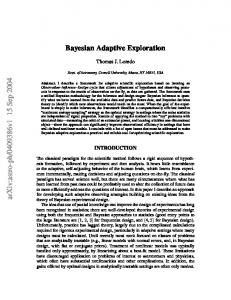
Figure 3: A. The FACETS user interface showing user exploration of the RottenTomatoes similar-movie graph. In the Exploration View (at 2), orange nodes are films traversed by the user. Exploring Brazil, the user selects it, highlighting its node in blue border (at 2), and its features in the Table View (at 1). Brazil has many neighbors (similar movies). The Neighborhood Summary (at 3) ranks them by measures like interest and surprise scores (left), and summarizes the neighborhood’s features (right). Global feature distributions are gray, local neighborhood distributions are orange. The distributions are shown as compact heat maps, expandable into histograms. Clicking a neighbor adds it to the Exploration View. The User Profile view (at 4) shows distribution summaries for the nodes explored thus far, to promote user understanding. B. Nodes are colored (at 2 & 3) based on their interest and surprise scores. More red means more user interest, more blue more surprising. A higher color saturation represents a higher score.

In Equation 2.2 we use base 2 so that 0 ≤ DJS (P ||G) ≤ 1. For a fresh node va, whose neighbors are not yet visualized we first compute the surprise-score, si, of all neighboring nodes vi ∈N(va): X (2.3) si = λj DJS (Li,j ||Gj ),

2.4 Ranking by Subjective Interestingness We track the user’s behavior and record a user profile as they explore their data. Each clicked node offers valuable details into the types of nodes in which the user is interested. This forms the user profile distribution Uj for each feature fj . To rank the user’s interest in the undisplayed neighbors of fj ∈A node va we follow a similar approach as in Equation 2.3: where Lj and Gj are the local and global distributions of nodeX ri = λj DJS (Li,j ||Uj ), feature fj and λj is a feature weight. Weighted feature scores in (2.5) fj ∈A Equation 2.3 are used to lessen the impact of noisy features and to allow the user to lessen the contribution of a feature manually. ˆa, which holds all the scores where Uj is the distribution of feature fj from the user’s recent The si scores are composed into S node browsing. In this case we want the local distributions that for the neighbors of initial node va. We find the most surprising match better the user’s current profile; i.e. we want the smallest k-nodes by looking for the largest divergence from the global: possible divergences: ˆa (2.4) argmaxS ˆa 1...k (2.6) argminR 1...k This yields the top-k most surprising nodes among the neighbors of node va. Since both the local-neighborhood and global feature This strategy suffers from the cold-start phenomenon, bedistributions are static, the surprise scores can be precomputed to cause a user will not have a profile until they have explored some improve real time performance. In our implementation, we pre- nodes, but it is possible to rank nodes only with surprise or concompute and store surprise in FACETS to improve performance. ventional measures, until the user has investigated several nodes.

600

Copyright © by SIAM Unauthorized reproduction of this article is prohibited

Downloaded 11/13/18 to 158.46.223.38. Redistribution subject to SIAM license or copyright; see http://www.siam.org/journals/ojsa.php

2.5 The FACETS Algorithm We summarize the process of finding top-k most interesting and surprising neighbors in our FACETS algorithm. Whenever a user selects a node to explore, we rank its neighbors based on surprise and subjective interestingness we explained in the previous subsections. For each of the neighbors, we compute surprise and interest scores for each feature and aggregate them based on feature weights λj . We blend those scores, and return the k nodes with highest scores. 3 The FACETS System We have developed FACETS, a scalable, interactive system that materializes our novel ideas for adaptive graph exploration. It enables users to explore real million-edge graphs in real time. This section describes how its visualization and interaction design works closely with its underlying computation to support user exploration. 3.1 Visualization & User Interface Design. FACETS’s user interface as shown in Figure 3 has four key elements: The first main area is (1) the Table View showing the currently displayed nodes and their features. This provides sortable node-level information. The central area is (2) the Exploration View. It is an interactive force-directed graph layout that demonstrates the structure and relationships among nodes as the user explores. Node colors are used to encode the surprise and interest based on the user’s current exploration. We have (3) the Neighborhood Summary to summarize neighbors, as we do not show a full set of neighbors in the Exploration View. The neighborhood summary allows users to investigate the feature distributions of its currently undisplayed neighbors as well as sort them by their interest or surprise scores. FACETS focuses on novel ranking measures. Conventional measures (e.g., PageRank, etc.) may also be available via the drop-down menu in Figure 3.3. This view presents the user with feature heat maps (darker colors represents higher values) which summarize the distributions of hidden nodes. When clicked, the heat maps turn into distribution plots (histograms), where a user can compare the local neighborhood (orange) and the global (gray). This lets a user quickly select new nodes based on their feature values and get a quick summary of this node’s neighborhood. As a user explores, we construct and display a summary profile of the important features they have covered in (4) the User Profile view. The user profile view suggests high-level browsing behavior to the user; allows for better understanding of where the user-interest ranking comes from; and allows them to adjust if they want to ignore certain features in the interest ranking. 3.2 Design Rationale We explain the rationale behind the design of FACETS in supporting exploration of large graphs. Exploring and Navigating One of our design goals is to facilitate both exploration and navigation of graphs. We use the term graph navigation to refer to the act of traversing graph

data with a known destination or objective. Graph exploration is more like foraging through the graph without a particular destination. We facilitate navigation through adaptation and exploration by filtering out unsurprising and unimportant nodes while still providing crucial feature details for hidden nodes via the Neighborhood Summary window. As shown in Figure 3.3, the user can bring up a summarized view of mouse-hovered nodes where the top ranked hidden neighbors, local distribution and global distribution are displayed. These neighborhood feature distributions allow quick and easy filtering. Show the Best First Keeping the graph view from becoming an incomprehensible mess of edges means only showing relevant, surprising, and interesting nodes. Importance, surprise, and user-interest are all important aspects of discovery, so we blend them into the results that are shown first to the user. Figure 3B illustrates how we visually encode the interest-surprise difference by hue and the sum of both scores by saturation. Nodes ranked high tend to have brighter color closer to purple, which becomes a clear visual cue for the user to quickly identify desired nodes. FACETS is almost completely free of parameters, making it simpler for users to explore their graphs. Adaptive and Adjustable Because user-interest varies greatly across users and even time, our design must be able to track the user’s exploration behavior in order to approximate what is motivating them. Adapting as the user explores helps provide critical insight into users’ latent objectives, because they can see how they have explored and also may find what they seek. During exploration, the user profile updates dynamically to illustrate a summary of their feature traversal, while the exploration view provides the topological traversal. It is not necessary to preset any parameters in order for our adaptive algorithm to work, because the rankings are done in a black-box fashion during users’ explorations. We allow them to directly manipulate the balance of features used in the interest calculation and choose which features form the ranking. This enables the user to dynamically increase or decrease the importance of any features during their exploration and immediately impact the interest ranking. 4 Evaluation We evaluate the effectiveness and speed of FACETS using large real-world graphs. FACETS is designed to support open-ended discovery and exploration suited to users’ subjective interests, which is inherently challenging to evaluate [8]. Traditional quantitative user studies (e.g., measuring task completion time) would impose artificial constraints that interfere with and even potentially suppress how users would naturally explore based on curiosity, counteracting the benefits that FACETS aims to foster. Given the exploratory nature of FACETS, canonical quantitative metrics of “success” like precision, recall, MAE, and RMSE [11, 33, 14] are not directly applicable here. For these reasons, we demonstrate FACETS’s effectiveness through several

601

Copyright © by SIAM Unauthorized reproduction of this article is prohibited

Downloaded 11/13/18 to 158.46.223.38. Redistribution subject to SIAM license or copyright; see http://www.siam.org/journals/ojsa.php

Network Rotten Tomatoes DBLP Google Web Youtube

Nodes

Edges

17,074 317,080 875,713 1,134,890

72,140 1,049,866 5,105,039 2,987,624

Obs. Study X

Speed X X X X

3. Exploration of movies, chosen by the participant, with consistent years (e.g., around mid 90’s)

Case Study X X

Table 2: Graph datasets used in our observational study, speed testing, and case studies. They were picked for their variety in size and domain. Rotten Tomatoes was used in the observational study due to its general familiarity to the public.

complementary ways: (1) a small observational study based on the study of exploratory systems from [8], (2) run time analysis of our surprise and interest rankings on four real world graphs, (3) a comparison of our scoring with canonical node ranking techniques, and three case studies that investigate the results of our algorithm on a movie graph and citation network. 4.1 Graph Datasets We use the Rotten Tomatoes (RT) movie dataset as our main dataset, which is an attributed graph that contains basic information per movie (e.g., released year), as well as users’ average ratings and critics scores. We conducted the observational study using the RT graph. We used four datasets for runtime analysis: RT graph, Google Web network, DBLP co-authorship graph, and YouTube network datasets [21]. Table 2 summarizes the graphs’ basic statistics and in which parts of our evaluation they were used. 4.2 Observational Study We conducted a small observational study with semi-structured interviews and surveys. Four participants were recruited through our institution’s mailing lists. We screened for participants with at least basic knowledge of movies (e.g., enjoy occasionally watching movies when they grew up). Three subjects were female and one was male, all had completed a bachelor’s degree. They ranged in age from 21 to 27, with an average age of 23. The participants were provided a 10-minute tutorial of FACETS, which demonstrated the different parts of FACETS and how they can be used to investigate the RT graph. They were asked to think aloud for the whole study, so that if they became confused or found something interesting we would be able to take notes. For all tasks, participants were free to choose movies to inspect, so that they would remain interested during their exploration. They could also look up movies on RottenTomatoes’ website if they were curious about details. Every participant performed three general tasks, each lasted for 10 minutes: 1. Open exploration of the RT graph to help acquaint the participants with FACETS 2. Investigation of the surprising neighbors of movies using the neighbor summary view (participants chose their own starting movies)

The first task was presented in order to encourage the participants to ask questions about the system, as well as investigate how they would use it without being directed. We were curious about which features they would use and if there were any behavioral patterns we could find during exploration. The second task was used to investigate quality of the surprising results. We let the participants pick their own starting movies since it would be easier for them to work with movies they knew. Our requirement was that the movie had at least five neighbors, so that the exploration options weren’t trivial. For the third task, we asked participants to choose and investigate a set of movies that interest them, with consistent years, so that they could see an example of how FACETS will adapt the interest ranking based on their recently clicked nodes. This task allowed the participants to comment on and better understand the interest ranking, and allowed us to get feedback on the quality of subjectively interesting results. The observations and feedback from the study allowed us to understand how FACETS’s visual encoding guides participants during exploration. 4.2.1 Observational Study Results We measured several aspects of FACETS using 7-point Likert scales (provided as a survey at the end of the study). The participants enjoyed using FACETS and additionally found that our system was easy to learn, easy to use and likeable overall; although this is a common experimental effect, we find the results encouraging. Users found both our rankings to be useful during their exploration. Several participants stated that the visualization combined with the interest and unexpectedness rankings to be very exciting during exploration. One participant stated, “it was exciting when I double clicked a node and saw how it was connected to my explored movies”. FACETS was able to find subjectively interesting content for our participants as they explored. Participants primarily spent time in two areas, on the main graph layout and in the neighborhood summary view. They used the neighborhood summary view to find and add new nodes and then inspected the relationships of these newly added nodes in the graph view. The table view was used primarily to select already-added nodes by name. Two participants reported not fully understanding how the user profile was affecting the results until the second task. The participants used a common strategy during exploration, in which they would add neighbors to a desired node and then spatially reorganize the results by dragging some of the new nodes to a clear area. They repeated this process and often inspected new nodes that shared edges with previous content. In summary, our design goal was generally met: our participants deem FACETS as an easy-to-learn and easy-to-use system with highly rated qualities of both interesting and unexpected neighborhood suggestions.

602

Copyright © by SIAM Unauthorized reproduction of this article is prohibited

Downloaded 11/13/18 to 158.46.223.38. Redistribution subject to SIAM license or copyright; see http://www.siam.org/journals/ojsa.php

Avg. Time (s) .08

Number of Features vs. Run Time 100 neighbors

.06

60 neighbors .04 .02 0

10 neighbors 10

20 30 #Features

40

50

Figure 5: FACETS scales linearly in the number of features

Figure 4: FACETS ranks neighbors in linear time and finishes in seconds. We show the average time to calculate the JS divergence for surprise and the combination of surprise and interest over a neighborhood of size n. FACETS combines the ranks if there is sufficient user profile data. We tested with contiguous node ordering to simulate normal exploration and random ordering to simulate a user searching using the table view.

4.3 Runtime Analysis Next, we evaluate the scalability of FACETS over several million-edge graphs (Table 2). Our evaluation focuses on demonstrating FACETS’s practicality in computing exploratory rankings in time that is linear in the number of neighbors and of node attributes, returning results in no more than 1.5 seconds for the 5 million edge Google Web graph that we tested. We expect these runtime results will significantly improve with future engineering efforts and optimization techniques. The experiments were run on a machine with an Intel i5-4670K at 3.65 GHz and 32GB RAM. One of our goals is sub-second rankings, so that interactions with FACETS are smooth. This is why we have chosen to treat nodes in the tail of the degree distribution separately than their modest degree neighbors. We have analyzed the runtime of FACETS, in Figure 4, using the graphs from Table 2; all but the RT graph used eight synthetic features. We use both random ordering and contiguous node ordering, displayed as Rand and Hop in Figure 4. Random ordering simulates using the search functionality while hop ordering simulates hopping from one node to its neighbors during exploration. High degree nodes have a higher chance of being selected and account for the fact that hop sometimes is slower than random in Figure 4. The graphs we tested demonstrate that the cost of the ranking is linear in the number of neighbors in the neighborhood. Our ranking requires both a value lookup and a single JS divergence calculation for each node and for each feature. As mentioned earlier, the surprise scores are precomputed

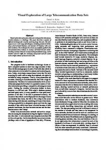
and can be accessed quickly. The cost to rank neighbors comes largely from the interest scores which cannot be precomputed. The cost, in JS divergence calculations, is O(n · f), and is asymptotically linear in both the number of neighbors n and the number of features f. Given our use of MDL histograms for the features, we can scale the number of features at low linear incremental cost (see Figure 5). Each neighbor only requires exactly one JS divergence calculation per feature (comparing the user profile and the local distribution). Since many real world graphs contain triangles, it is very likely that redundant calls will be made during a user’s exploration. We use this to our advantage and cache the distributions for each visited node rather than refetching them each time. Graphs with higher clustering coefficient may achieve better caching performance. For all but the YouTube graph, the caching became memoizing as the entirety of the nodes could fit in the cache. 4.4 Case Study We present a case study using the DBLP co-authorship graph to illustrate how FACETS helps users explore graphs incrementally, gain understanding, and discover new insights. DBLP Example: Data mining and HCI researchers This example uses data collected from DBLP, a computer science bibliography website. The graph is an undirected, unweighted graph describing academic co-authorship. Nodes are authors, and an edge connects two authors who have co-authored at least one paper. Our user Jane is a first-year graduate student new to data mining research. She just started reading seminal articles written by Philip Yu (topmost orange node in Figure 6). FACETS quickly helps Jane identify other prolific authors in the data mining and database communities, like Jiawei Han, Rakesh Agrawal, Raghu Ramakrishnan, and Christos Faloutsos; these authors have similar feature distributions as Philip Yu (e.g., very high degree). Jane chooses to further explore Christos Faloutsos’s co-authors. FACETS suggests Duen Horng Chau as one of the surprising co-authors, who seems to have relatively low degree (i.e., few publications) but has published with highly-prolific co-authors.

603

Copyright © by SIAM Unauthorized reproduction of this article is prohibited

Degree of Interest The visualization community has also investigated local graph exploration to handle very large graphs [30, 1, 36, 24]. Bottom-up exploration first appeared in [12], a tool for exploring hierarchies using a “degree of interest” (DOI) function to rank the relevance of currently undisplayed nodes. The idea of DOI was later expanded by [30] to apply to a greater set of graph features. The Apolo system [5] further improves on it to allow users to freely define their own arbitrary number of clusters, which it uses to determine what to show next, through the Belief Propagation algorithm. Recently, the DOI idea is applied to dynamic graph settings, to capture salient graph changes [1]. We have built on the idea of using a DOI to determine the ranking for which nodes we show users; however, we use a dynamic DOI function which changes to suit the browsing behavior of the users as they explore their data.

Interesting

Downloaded 11/13/18 to 158.46.223.38. Redistribution subject to SIAM license or copyright; see http://www.siam.org/journals/ojsa.php

Philip S. Yu Christos Faloutsos

Jiawei Han Jeffrey F. Naughton

Raghu Ramakrishnan Rakesh Agrawal Duen Horng Chau

Surprising Mary Beth Rosson Brad A. Myers James A. Landay Scott E. Hudson Gregory D. Abowd

John M. Carroll Chris North

Ben Shneiderman

Catherine Plaisant

Interesting

Interesting

Figure 6: Visualization of our user Jane’s exploration of the DBLP co-authorship graph. Jane starts with Philip Yu. FACETS then suggests Christos Faloutsos and several others as prolific data mining researchers. Through Christos, FACETS suggests Duen Horng Chau as a surprising author as he has published with both data mining and human-computer interaction (HCI) researchers, like Brad Myers. Through Brad, FACETS helps Jane discover communities of HCI researchers, including Ben Shneiderman, the visualization guru.

Among these is Brad Myers (leftmost orange node in Figure 6), who publishes not in data mining, but in human-computer interaction (HCI). This exploration introduces Jane to a new field, and she wants to learn more. Using FACETS’s interest-based suggestion, she discovers a community of co-authors who have published with Brad; among them, Mary Beth Rosson further leads to another community of HCI researchers, which includes Ben Shneiderman, the visualization guru. 5 Related Work Graph Trails and Paths In information retrieval. click trail analysis has been used to analyze the website-to-website paths of millions of users in order to improve the ranking of search results [4, 27, 35]. Intermediate sites and destinations of common trails can be included in search results. West et al. analyzed Wikipedia users’ abilities and common patterns as they explored Wikipedia [34]. They observed that users would balance between a conceptually simple solution at the cost of efficiency – users may take routes that are longer but easy to comprehend. Their system also used trail analysis in order to try to predict where a user would go based on the user’s article-trail features. In our case, we do not have millions of explored paths through our input network and cannot directly rely on the aggregate analysis of trails used above.

Surprise and Serendipity Many fascinating works point to the great potential in leveraging surprise and serendipity [3, 6, 7, 22, 31]. Realizing that applying them on graph exploration could be a novel and practical idea, we decided to focus on studying them in this work as they are under-explored, unlike conventional importance-based metrics [1, 5, 30]. Algorithms like Oddball [2], an unsupervised approach to detect anomalies in weighted graphs, can be used to detect surprising nodes. The TANGENT algorithm by Onuma et al. [22] is a parameter-free technique used to discover surprising recommendations by measuring how broadly new nodes expand edges to new clusters. Similar to our approach, several researchers have developed methods to measure interestingness based on comparing data distributions. Vartak et al. [31] presented the idea of finding interesting visualizations based on an underlying database query. Andre et al. [3] studied the use of serendipity in Web search and the effects of personalization. They found that serendipity and personalization could be useful for many queries, ideas which we leverage in FACETS. De Bie [6, 7] proposed a general framework for measuring the interestingness of data mining results as their log-likelihood given a Maximum Entropy distribution based on user’s background knowledge. Instead, we consider the Jensen-Shannon divergence between the local and global histograms as the surprisingness of a node. Our notion of subjective interestingness comes closer to that of Tatti and Vreeken [28], who aimed to reduce data redundancy. Our goal is different, as we are specifically interested in identifying nodes and neighborhoods that are similar to those the user chose to explore. 6 Conclusion We presented FACETS, an integrated approach that combines visualization and computational techniques to help users perform adaptive exploration of large graphs. FACETS overcomes many issues commonly encountered when visualizing large graphs by showing the users only the most subjectively interesting material as they explore. We do this by ranking the neighbors of each node by surprisingness (divergence between local features

604

Copyright © by SIAM Unauthorized reproduction of this article is prohibited

Downloaded 11/13/18 to 158.46.223.38. Redistribution subject to SIAM license or copyright; see http://www.siam.org/journals/ojsa.php

and global features) and subjective interest based on what the user has explored so far (divergence between local features and user profile). To evaluate the effectiveness of FACETS, we used several complementary ways. Our FACETS algorithm is scalable and is linear in the number of neighbors and linear in the number of features. Participants in a small observational study consistently rated FACETS well. References [1] J. Abello, S. Hadlak, H. Schumann, and H.-J. Schulz. A modular degree-of-interest specification for the visual analysis of large dynamic networks. IEEE TVCG, 20(3):337–350, 2014. [2] L. Akoglu, M. McGlohon, and C. Faloutsos. Oddball: Spotting anomalies in weighted graphs. In PAKDD, pages 410–421. Springer, 2010. [3] P. Andr´e, J. Teevan, and S. T. Dumais. From x-rays to silly putty via uranus: serendipity and its role in web search. In SIGCHI, pages 2033–2036. ACM, 2009. [4] M. Bilenko and R. W. White. Mining the search trails of surfing crowds: Identifying relevant websites from user activity. In WWW, pages 51–60. ACM, 2008. [5] D. H. Chau, A. Kittur, J. I. Hong, and C. Faloutsos. Apolo: interactive large graph sensemaking by combining machine learning and visualization. In KDD, pages 739–742. ACM, 2011. [6] T. De Bie. An information theoretic framework for data mining. In KDD, pages 564–572. ACM, 2011. [7] T. De Bie. Maximum entropy models and subjective interestingness: an application to tiles in binary databases. Data Min. Knowl. Disc., 23(3):407–446, 2011. [8] M. D¨ork, N. H. Riche, G. Ramos, and S. Dumais. Pivotpaths: Strolling through faceted information spaces. TVCG, 18(12):2709–2718, 2012. [9] N. Elmqvist, T. N. Do, H. Goodell, N. Henry, and J. D. Fekete. Zame: Interactive large-scale graph visualization. In 2008 IEEE Pacific Visualization Symposium, pages 215–222, March 2008. [10] M. Faloutsos, P. Faloutsos, and C. Faloutsos. On power-law relationships of the internet topology. In SIGCOMM, volume 29, pages 251–262. ACM, 1999. [11] F. Fouss, A. Pirotte, J.-M. Renders, and M. Saerens. Randomwalk computation of similarities between nodes of a graph with application to collaborative recommendation. IEEE TKDE, 19(3):355–369, March 2007. [12] G. W. Furnas. Generalized fisheye views. SIGCHI Bull., 17(4):16–23, Apr. 1986. [13] T. H. Haveliwala. Topic-sensitive pagerank. In WWW, pages 517–526, New York, NY, USA, 2002. ACM. [14] J. L. Herlocker, J. A. Konstan, L. G. Terveen, and J. T. Riedl. Evaluating collaborative filtering recommender systems. TOIS, 22(1):5–53, 2004. [15] Y. Jia, J. Hoberock, M. Garland, and J. Hart. On the visualization of social and other scale-free networks. IEEE TVCG, 14(6):1285–1292, Nov 2008. [16] S. Kairam, N. H. Riche, S. M. Drucker, R. Fernandez, and J. Heer. Refinery: Visual exploration of large, heterogeneous networks through associative browsing. Comput. Graph. Forum, 34(3):301–310, 2015.

[17] D. A. Keim. Visual exploration of large data sets. Commun. ACM, 44(8):38–44, 2001. [18] D. A. Keim. Information visualization and visual data mining. TVCG, 8(1):1–8, 2002. [19] P. Kontkanen and P. Myllym¨aki. MDL histogram density estimation. In AISTATS, 2007. [20] T. Lee, Z. Wang, H. Wang, and S. won Hwang. Attribute extraction and scoring: A probabilistic approach. In ICDE, pages 194–205, 2013. [21] J. Leskovec and A. Krevl. SNAP Datasets: Stanford large network dataset collection. http://snap.stanford.edu/data, June 2014. [22] K. Onuma, H. Tong, and C. Faloutsos. Tangent: a novel,’surprise me’, recommendation algorithm. In KDD, pages 657–666. ACM, 2009. [23] L. Page, S. Brin, R. Motwani, and T. Winograd. The pagerank citation ranking: Bringing order to the web. Technical report SIDL-WP-1999-0120, Stanford, 1999. [24] R. Pienta, J. Abello, M. Kahng, and D. H. Chau. Scalable graph exploration and visualization: Sensemaking challenges and opportunities. In International Conference on Big Data and Smart Computing, pages 271–278. IEEE, 2015. [25] C. Plaisant, B. Milash, A. Rose, S. Widoff, and B. Shneiderman. Lifelines: visualizing personal histories. In SIGCHI, pages 221–227. ACM, 1996. [26] B. Shneiderman. The eyes have it: A task by data type taxonomy for information visualizations. In VL, pages 336–343. IEEE, 1996. [27] A. Singla, R. White, and J. Huang. Studying trailfinding algorithms for enhanced web search. In SIGIR, pages 443–450. ACM, 2010. [28] N. Tatti and J. Vreeken. Comparing apples and oranges measuring differences between exploratory data mining results. Data Min. Knowl. Disc., 25(2):173–207, 2012. [29] H. Tong, C. Faloutsos, and J.-Y. Pan. Fast random walk with restart and its applications. In ICDM, pages 613–622. IEEE, 2006. [30] F. Van Ham and A. Perer. Search, show context, expand on demand : Supporting large graph exploration with degree-of-interest. TVCG, 15(6):953–960, 2009. [31] M. Vartak, S. Rahman, S. Madden, A. Parameswaran, and N. Polyzotis. Seedb: efficient data-driven visualization recommendations to support visual analytics. PVLDB, 8(13):2182–2193, 2015. [32] T. Von Landesberger, A. Kuijper, T. Schreck, J. Kohlhammer, J. J. van Wijk, J.-D. Fekete, and D. W. Fellner. Visual analysis of large graphs: state-of-the-art and future research challenges. In Computer graphics forum, volume 30, pages 1719–1749. Wiley Online Library, 2011. [33] F. Wang, S. Ma, L. Yang, and T. Li. Recommendation on item graphs. In ICDM, pages 1119–1123, Dec 2006. [34] R. West and J. Leskovec. Human wayfinding in information networks. In WWW, pages 619–628. ACM, 2012. [35] R. W. White and J. Huang. Assessing the scenic route: Measuring the value of search trails in web logs. In SIGIR, pages 587–594. ACM, 2010. [36] K.-P. Yee, D. Fisher, R. Dhamija, and M. Hearst. Animated exploration of dynamic graphs with radial layout. In IEEE Symposium on Information Visualization, 2001.

605

Copyright © by SIAM Unauthorized reproduction of this article is prohibited