Appears in PLDI '01
Facile: A Language and Compiler For High-Performance Processor Simulators1 Eric C. Schnarr
Mark D. Hill
James R. Larus
QUIQ Incorporated 25 Kessel Court, Suite 201 Madison, WI 53711
University of Wisconsin—Madison 1210 West Dayton Street Madison, WI 53706
Microsoft Research One Microsoft Way Redmond, WA 98052
[email protected]
[email protected]
[email protected]
ABSTRACT
1. INTRODUCTION
Architectural simulators are essential tools for computer architecture and systems research and development. Simulators, however, are becoming frustratingly slow, because they must now model increasingly complex micro-architectures running realistic workloads. Previously, we developed a technique called fast-forwarding, which applied partial evaluation and memoization to improve the performance of detailed architectural simulations by as much as an order of magnitude [14].
Detailed simulation is an essential tool for computer architecture and systems research and development. As computers, in particular processor micro-architectures, have become increasingly complex, so have their simulators. While this complexity has greatly improved processor performance, it has had the opposite effect on simulator speed. Complex simulators run slowly, which impairs their usefulness in evaluating processor implementations or developing software. Moreover, architecture simulators are complex pieces of software that are difficult to write, debug, and validate.
While writing a detailed processor simulator is difficult, implementing fast-forwarding is even more complex. This paper describes Facile, a domain-specific language for writing detailed, accurate micro-architecture simulators. Architectural descriptions written in Facile can be compiled, using partial evaluation techniques, into fast-forwarding simulators that achieve significant performance improvements with far less programmer effort. Facile and its compiler make this performance-enhancing technique accessible to computer architects.
Categories and Subject Descriptors D.3.2 [Programming Languages]: Language Classifications— specialized application languages; D.3.4 [Programming Languages]: Processors—optimization, compilers; D.3.3 [Programming Languages]: Language Constructs and Features— constraints, frameworks; I.6.2 [Simulation and Modeling] Simulation Languages.
General Terms Algorithms, Languages, Performance.
Keywords Micro-architecture simulation, out-of-order processor simulation, memoization, and partial evaluation.
Copyright © 2001 by the Association for Computing Machinery, Inc. Permission to make digital or hard copies of part or all of this work for personal or classroom use is granted without fee provided that copies are not made or distributed for profit or commercial advantage and that copies bear this notice and the full citation on the first page. Copyrights for components of this work owned by others than ACM must be honored. Abstracting with credit is permitted. To copy otherwise, to republish, to post on servers, or to redistribute to lists, requires prior specific permission and/or a fee. Request permissions from Publications Dept., ACM Inc., fax +1 (212) 869-0481, or
[email protected].
1
Facile—our domain-specific language for writing detailed processor architecture simulators—attacks both problems, with a goal of making efficient simulators more accessible to computer architects. We previously showed that programming language implementation techniques—partial evaluation and memoization— could increase simulator performance by up to an order of magnitude [14]. This approach, called fast-forwarding, was very difficult to implement by hand, which led to this research on the Facile language for describing instruction encodings, instruction semantics, and micro-architectural details and on the Facile compiler for translating a processor description into an efficient simulator. The compiler uses partial evaluation analyses to translate a simulator written in Facile into a fast-forwarding simulator, which uses runtime partial evaluation to greatly improve performance [13]. Instruction-level simulation focuses on modeling instructions’ effect on user-visible state; for example, that an add instruction puts the sum of two registers into a third. These simulators typically are interpreters, written in a procedural language such as C, that read instructions from a target executable and execute their functional behavior. Many approaches have been tried to accelerate this process. Some simulators pre-decode target instructions, to make interpretation easier, e.g., SPIM [6] and SimICS [10]. Others compile target instructions into native host instructions and then directly execute them, e.g., FX!32 [2] and Shade [3]. Architectural or micro-architectural simulation, by contrast, simulates the behavior of a processor implementation by modeling instructions’ effects on processor structures. For example, the registers used by the add instruction might be dynamically renamed and the add operation dynamically scheduled on one of several 1. This work was largely performed as part of Eric Schnarr's Wisconsin Ph.D. [13]. It was supported in part by the National Science Foundation with grants MIP-9625558 and EIA-9971256.
Appears in PLDI '01
ALUs. Modern, out-of-order processors are built on complex micro-architectures, whose simulation is very expensive. SimpleScalar, a fast, popular out-of-order simulator, incurs approximately a 4,000 times slowdown [1]. RSIM, an out-of-order multiprocessor simulator, executes fewer than 15,000 instructions per second on a SUN Ultra 1/140 workstation, which is approximately a 10,000 times slowdown per processor [11]. MXS, the SimOS out-of-order simulator, also incurs a several thousand times slowdown per processor [7]. Techniques that enhance functional simulators offer little benefit for architectural simulators, most of whose time is spent simulating an out-of-order pipeline, not interpreting instructions. Fortunately, simulators, like compilers and computer architectures, can exploit program locality to improve performance. Even detailed out-of-order simulators spend most of their time modeling a small number of instruction sequences. Run-time partial evaluation and memoization permit the rapid re-simulation of these sequences. This approach is the basis of our fast-forwarding technique. Writing fast-forwarding simulators is difficult. A programmer must not only understand and correctly model a processor’s microarchitecture, but he or she must also distinguish run-time static and dynamic data; implement two, tightly-coupled simulation engines; and ensure that both appropriately model simulator state. Facile is a new domain-specific programming language for writing fast-forwarding simulators. It is designed to facilitate the specification and implementation of detailed architecture simulators and to simplify the compiler analyses necessary to automatically produce a fast-forwarding simulator. For example, a simulator for the SPARC V9 instruction set running on a MIPS R10000-like out-oforder processor requires less than 2,000 lines of Facile and another 1,000 lines of C code. The Facile compiler uses a new approach to the classic problem of partial evaluating an interpreter for a given input program [8]. Unlike much partial evaluation work, fast-forwarding occurs at run time. In many respects, Facile is similar to run-time specialization and code generation systems, though Facile’s domain-specific language and limited application domain permits a very fine-grain and aggressive translation that results in large performance gains. The rest of this paper is organized as follows. Section 2 describes how memoization works to speed micro-architecture simulation. Section 3 introduces Facile, our new programming language, and discusses how it supports fast-forwarding simulators. Section 4 describes how Facile’s compiler analyzes and optimizes simulators. Section 5 discusses related work. Section 6 presents the performance of a hand-coded out-of-order simulator and an out-oforder simulator optimized by the Facile complier.
2. FAST-FORWARDING Fast-forwarding is an application of partial evaluation and memoization to micro-architecture simulation. This basic execution model was described previously [14]. Fast-forwarding improved the performance of a detailed out-of-order processor simulator 5–12 times over the same simulator without memoization. Below is a brief description of this technique, which provides the run-time framework for this work.
2
Slow/Complete Simulator
Specialized Action Cache
lookup static input
recover from memoization miss
Fast/Residual Simulator Figure 1. Architecture of a fast-forwarding simulator.
2.1. Overview The basic idea is to capture a simulator’s computation of an instruction’s effects on processor micro-architecture in a form that can be rapidly re-executed. For example, an out-of-order simulator might record timing and functional effects of one processor cycle, indexed by the collection of instructions in execution at the start of the cycle. This example is explored in Section 2.2. Recorded effects can be quickly re-executed without interpretive overhead or the need to re-compute, as opposed to simply re-applying, instructions’ effects on processor state. Most simulators can be modeled as a simulator step function. Each call to this function advances the simulation by a single step. A simulator’s author determines the amount of calculation performed in a step, which can range from simulating one processor cycle to simulating several cycles and instructions. The simulator step function’s implementation determines the granularity of memoization, since calls on this function are memoized. If one instruction is simulated per step, the behavior of individual instructions can be looked up and replayed. If several instructions are simulated per step, their combined behavior can be replayed when the same group of instructions is encountered. Consider a simulator step function f. This function takes as input the state of the simulated micro-architecture and returns a new state that reflects the execution of one simulation step. To fast-forward f, part of its input (i.e., a subset of the micro-architecture state) is designated run-time static (constant) and used to index a cache of specialized actions: f : ( S in × D in ) → D out As shown above, f’s input is divided into run-time static input (Sin) and dynamic input (Din). Run-time static input typically includes the binary instructions being simulated and a subset of the processor pipeline state. Dynamic inputs usually include values in simulated registers, addresses resident in a simulated data cache, etc. All code in f that depends only on Sin is also run-time static, so that in any two calls to f that are passed the same values for Sin, f’s runtime static code produces the same result. Only code that depends on dynamic data (Din) can produce a different result.
Appears in PLDI '01
Action cache entry
slow simulation. To recover from the miss, this simulator rolls back the failed dynamic step function, reads its static input from the cache entry’s index key, and restarts the slow simulator step function. This simulator executes the new control flow path, recording its actions, so that the new control flow path can be replayed in the future.
Key (run-time static inputs)
?
?
? ?
Missing control paths
Dynamic actions Figure 2. The specialized action cache. When a fast-forwarding simulator encounters a particular run-time static input (Sin) for the first time, it both executes f to effect the simulation and uses partial evaluation to specialize f with respect to Sin. The specialized function, f Sin : D in → D out , is stored into a specialized action cache, indexed by Sin. Subsequent calls to f, with input Sin, execute the less expensive function fSin instead of f. Figure 1 depicts the architecture of a fast-forwarding simulator. At the top is the slow/complete simulator, which consists of the unspecialized simulator step function. As the slow simulator executes, it writes a description of its dynamic behavior—the partially evaluated function fSin—into the specialized action cache. When the step function encounters a previously seen run-time static input, the dynamic behavior is found and replayed by a fast/residual simulator. A replayed simulation can only re-execute a previously recorded control flow path. While replaying, the fast simulator verifies that the control flow path is known and re-executes actions associated along the path. If the path is not cached, an action cache miss returns control to the complete simulator. This process is a dynamic version of the classic partial evaluation of an interpreter for an input program [8]. An important difference is that fast-forwarding is a run-time process. Another difference is that traditional partial evaluation systems generate residual code for an entire function, which is not feasible because simulator step functions are large and must be specialized for many different inputs. Fast-forwarding addresses these concerns by specializing only control flow paths executed by the slow simulator and by specializing these paths on demand. Because of the high degree of locality in program execution, the specialized action cache remains a manageable size and actions are heavily reused [14]. Figure 2 illustrates the structure of the specialized action cache. It contains cache entries, which consist of index keys—the step function’s run-time static input—and the simulator’s residual dynamic actions. Actions are linked together in the order in which they execute. Actions that select control-flow paths, by examining dynamic values, have multiple successors. The simulator records its actions when it executes a control flow path, so successors of an action may be missing. For example, a branch that was previously always taken will have no recorded behavior for the fall-through case. When the fast simulator encounters a missing action, it incurs an action cache miss and returns to
3
Recovery from a miss is complicated. Fast simulation may already have moved beyond the beginning of the simulator’s step function (i.e., the location of a key in the specialized action cache), and modified dynamic simulator state, before encountering the miss. Intuitively, the dynamic state should be rolled back to the beginning of the step function call, but this is not always possible. Instead of rolling the fast simulation back, the slow simulator proceeds cautiously and does not execute dynamic actions until it reaches the cache miss. Until then, the slow simulator only performs run-time static operations and stores no new data into the specialized action cache. After reaching the cache miss, the slow simulator returns to normal execution, executing both run-time static and dynamic code and adding new actions to the cache.
2.2. Example: Out-Of-Order Simulation Fast-forwarding is very effective at accelerating the simulation of a modern, out-of-order micro-architecture. One implementation uses a simulator step function that takes the current state of the out-oforder pipeline as its run-time static input and simulates the microarchitecture until the end of a processor cycle that performs some dynamic behavior. This approach allows the fast simulator to skip over most cycle-by-cycle pipeline simulation, replaying only functional instruction behavior and other non-pipeline simulation such as branch prediction and cache simulation. Our simulator encodes the run-time static state of an out-of-order pipeline in a data structure called the instruction queue. The instruction queue does not correspond to any micro-architecture component. It is simply a convenient data structure for representing run-time static data. The instruction queue is a list of instructions, in program order, currently in execution. A small amount of additional information specifies the pipeline stage and latency of each instruction, e.g., fetched, waiting in out-of-order queue, executing, etc. The left side of Figure 3 shows an example of data in the instruction queue. The first 11 instructions are in the instruction queue. Over the next 6 simulated cycles, only run-time static behavior occurs: the first instruction (clr) is retired, 9 more instructions are fetched, several instructions use the simulated ALUs2, and the load (ld) instruction at address 0x10078 counts down to the next time it needs to make a dynamic call to the cache simulator. The right side of Figure 3 shows data in the specialized action cache for this pipeline state. An entry’s key consists of a compressed representation of the instruction queue. The instruction queue in this example can be compressed into fewer than 40 bytes, since its contents can be reconstructed from the underlined values. The first action increments the simulated cycles by 6, for the 6 2. In this example, the functional simulation of instructions is dynamic, but separate from micro-architectural timing simulation. Instructions are first interpreted for their functional behavior, then their pipeline timing is simulated.
Appears in PLDI '01
Previous Action Out-Of-Order Pipeline State Addr. 0x10074 0x10078 0x1007c 0x10080 0x10084 0x10088 0x1008c 0x10098 0x1009c 0x100a0 0x100a4 0x3f378 0x3f380 0x3f384 0x3f388 0x56ce8 0x56cec 0x56cf0 0x56cf4 0x56cf8
Instruction clr %fp ld [ %sp + 0x40 ], %l0 add %sp, 0x44, %l1 sub %sp, 0x20, %sp tst %g1 be 0x10098 mov %g1, %o0 sethi %hi(0x5b000), %o0 or %o0, 0x148, %o0 call 0x3f378 nop save %sp, -96, %sp sethi %hi(0x75c00), %o0 call 0x56ce8 or %o0, 0x2e0, %o0 save %sp, -96, %sp sethi %hi(0x77000), %g1 ld [ %g1 + 0x17c ], %g1 call %g1 restore
Stage done cache exec queue queue queue queue fetch fetch fetch fetch
Latency
Action Cache Entry
Key Compressed
6 1
Pipeline State 16+11*2 = 38 bytes
Add 6 to cycle counter
Call cache simulator for load at 0x10078 Memory cache miss
delay=18
Next Action
Memory cache hit
Unknown
Figure 3. An out-of-order pipeline state with SPARC instructions and resulting specialized action cache entries. cycles of run-time static execution. The next action calls the cache simulator for the load at address 0x10078. The cache simulator has multiple possible results corresponding to a cache hit or miss. In this example, the load previously missed in the cache and waited 18 cycles before checking if the value was returned from the next level of the cache hierarchy. Subsequent fast simulation can replay these actions, so long as the load again misses in the cache with an 18-cycle delay. If during replay, the load hits in the cache (or misses with a different delay), then it is an action cache miss and control returns to the slow simulator.
3. FACILE LANGUAGE As the previous discussion probably made clear, writing fast-forwarding simulators is difficult. A programmer must not only understand and correctly model a processor’s micro-architecture, but he or she must also distinguish between run-time static and dynamic data; implement two, tightly-coupled simulation engines; ensure that simulator state is appropriately modeled by each; and transfer control and state between them. Facile is a new domain-specific programming language for writing fast-forwarding micro-architecture simulators. It is designed to facilitate the specification and implementation of detailed architecture simulators and to simplify the compiler analyses necessary to automatically generate a fast-forwarding simulator. Section 3.1 discusses Facile’s syntax for describing machine instructions and illustrates its use in a simple example. Section 3.2 discusses Facile’s support for partial evaluation and memoization.
4
This support includes language restrictions to simplify compiler analyses and a framework for writing simulators as step functions.
3.1. Architecture Description Facile provides a concise syntax for describing a computer’s architecture and instruction set. This syntax is partially derived from the New Jersey Machine Code Toolkit’s description language [12]. This language was the starting point for Facile’s instruction description syntax, because its descriptions are concise, designed to reduce programmer error, and flexible enough to describe instruction sets ranging from RISC to Intel x86. Facile extends this work to include instruction semantics, as well as syntax. Facile describes binary encoding of instructions using patterns on streams of fixed width tokens. Figure 4 illustrates a Facile token, field, and pattern declarations. These declarations describe the encoding of two instructions, add and bz (branch if zero), of a fictitious RISC ISA. A token declaration defines one fixed width
token instruction[32] fields op 24:31, r1 19:23, r2 14:18, r3 0:4, i 13:13, imm 0:12, offset 0:18, fill 5:12; pat add = op==0x00 && (i==1 || fill==0); pat bz = op==0x01; Figure 4. Instruction encoding in Facile.
Appears in PLDI '01
val PC : stream; val nPC : stream; val R = array(32){0};
val init = system?start_pc; fun main(pc) { PC = pc; // set global PC variable nPC = PC + 4; // default value for npc PC?exec(); // simulate 1 instruction init = nPC; // prepare next iteration } Figure 6. Simplified simulator step function.
sem add { if(i) R[r1] = R[r2] + imm?sext(32); else R[r1] = R[r2] + R[r3]; }; sem bz { if(R[r1]==0) nPC = PC + offset?sext(32); }; Figure 5. Instruction semantic description.
tional and architectural behavior. This function is called from a user-defined simulator step function.
3.2. Language Support For Fast-Forwarding
token and names several bit fields contained within that token. The op field in Figure 4 is contained in bits 24 to 31 of a 32-bit wide token named instruction. For fixed width instruction sets, such as SPARC and MIPS, one token suffices to encode each instruction. For variable width instructions, such as Intel’s x86, several tokens may be necessary. Pattern declarations associate mnemonic names with conditions on token fields and use these constraints to describe instructions. In Figure 4, the add and bz pattern names are associated with values 0x00 and 0x01 respectively in an instruction’s op field. The add instruction has additional conditions: Either the immediate flag field (i) must be 1 or bits 5 through 12 (the fill field) must be 0. A token stream is a sequence of tokens starting at an address in the text segment of a simulated executable. The instruction at the front of a token stream is decoded by matching the binary data at that location against a pattern. Unlike the NJ Machine Code Toolkit, Facile describes instruction semantics as well as instruction encoding. Figure 5 shows the semantics of the add and bz instructions from Figure 4. First, global variables PC, nPC, and R are declared. PC and nPC are token stream variables that represent the current program counter and the program counter of the next instruction, respectively. R is an array of integers that holds the contents of the integer register file. Next, semantic declarations associate functional simulation code with the pattern names add and bz. Instruction add tests the value of the i field: if i is 1, then it adds an integer register to the instruction’s sign extended immediate field (imm). Otherwise, it adds two integer registers. The added result is written back to the integer register file. Instruction bz tests if an integer register is 0, and alters the next instruction address if true. The semantic code associated with each instruction can perform micro-architecture simulation and other tasks in addition to behavioral simulation. The Facile language provides functions, loops, arrays, and other general programming constructs. These programming features were included in Facile because no single, specialpurpose micro-architecture declarative syntax seemed likely to be able to model all possible micro-architecture structures. Given encoding and semantic functions, the Facile compiler automatically generates a function that decodes a binary instruction, dispatches to the appropriate simulation code, and simulates func-
5
Facile’s support for fast-forwarding starts with its organization of simulator code into a step function. Facile programmers define a function named main to perform one step in the simulation. This step can simulate one or more processor cycles, one or more instructions, or any other appropriate simulation quantum. Facile’s run-time system repeatedly calls main to advance the simulation. Calls to main are memoized. The main function receives two kinds of input: run-time static input is passed as arguments to main. Dynamic input comes from other sources, such as global variables or from external code not written in Facile. The arguments to main are the run-time static keys into the specialized action cache. The programmer defines the number and type of main’s arguments and controls exactly what data values are passed to them. Figure 6 shows a trivial simulator step function that simulates one target instruction per call. A global variable (init) stores argument values for the next call to main. At the start of simulation, init is set to the target program’s entry point (start_pc). This main function has one run-time static input (pc), whose initial value comes from init. The body of main copies pc into global variable PC for use by the simulation code, predicts the value of nPC (branch instructions may reset it), and simulates one target instruction. The last statement in main updates init with the pc for the next call to main. Facile has several other features that support writing fast-forwarding simulators. These include built-in data structures and functions useful for micro-architecture simulation, and language restrictions that simplify compiler analysis. The built-in data types include token streams, condition code values (with functions for computing them), and double-ended queues useful for modeling microarchitectures. By including these functions and data types into the language, their semantics are known, so a compiler can analyze and transform code that uses them. One built-in support function is the ?exec() attribute used in Figure 6. The ?exec() attribute is applied to a token stream (PC) and uses the declared tokens, patterns, and instruction semantics to decode and simulate one instruction. A key language restriction is the absence of pointers, which increases the precision of the analysis that determines which parts of a simulator step function can be skipped by fast-forwarding. Another restriction is the absence of recursion. Non-recursive code simplifies inter-procedural analyses. It also simplifies the mechanism for recovering from action cache misses, by allowing
Appears in PLDI '01 executable’s text segment3. Variables assigned a run-time static value are labeled rt-static until they are re-assigned. Hence, npc is rt-static because it depends only on the rt-static values pc and 4.
fun main(pc) { val npc = pc + 4; switch(pc) { pat add: if(i) R[r1] = R[r2] + imm?sext(32); else R[r1] = R[r2] + R[r3]; pat beq: if(R[r1] == 0) npc = pc + offset?sext(32); } init = npc; } Figure 7. Run-time static and dynamic code (underlined).
Code is labeled dynamic when it depends on dynamic data. In the example, the statement adding a register to an immediate, the statement adding a register to another register, and the condition testing a register against the value 0 are dynamic. Sub-expressions (not underlined) in these statements that are rt-static (e.g., register indices and the added immediate value) are skipped by fast-forwarding, even though the statements containing them are not.
dynamic data to be passed from the fast simulator to the slow simulator in global variables, not a stack. Facile is sufficiently powerful to model a real instruction set and complex processor implementation. It has been used to describe the SPARC-V9 instruction set and a detailed, out-of-order pipeline with non-blocking data caches, branch prediction, and speculative execution. Code that is inconvenient in Facile, or that need not be memoized, can be implemented in other languages, such as C. Facile provides an interface for calling external code, and memoizes Facile code correctly despite calls on external functions.
4. COMPILATION AND OPTIMIZATION The Facile compiler generates an optimized fast-forwarding simulator. The compiler actually generates C code for two simulators— slow and fast—and generates code to coordinate their communication through the specialized action cache. This process relies on binding-time analyses to identify run-time static code and dynamic basic blocks. The analyses and code generation are described below.
4.1. Binding-Time Analysis Binding-time analysis is a technique widely used in partial evaluation to partition a function’s code into static and dynamic parts, starting from an initial division of a function’s input. In Facile, binding-time analysis divides a simulator step function into runtime static and dynamic parts. The run-time static code is a function of the run-time static input, so its computation can be memoized and skipped by fast-forwarding. The remaining dynamic code, on the other hand, must be executed every time. Figure 7 shows the division of a Facile main function into runtime static and dynamic parts. Dynamic code is underlined. All other code is run-time static. Note that this function performs the same actions as the main function in Figure 6, except that instruction semantic code is written as a pattern switch statement for greater clarity. Binding-time analysis performs an abstract interpretation of the code, computing two binding time labels—rt-static and dynamic— instead of actual data values. At the beginning of this interpretation, the arguments to main (pc) and literal values (e.g., 4) are labeled rt-static and all global variables are labeled dynamic. The basic step is to label rt-static the result of expressions whose operands are all rt-static. For example, the switch statement is rt-static because it depends only on the rt-static values of pc and the target
6
Other complications are not exposed by this example, such as assignment to global variables. In Figure 7, assignment to init is labeled dynamic because its value is needed after main returns. In other cases, a global variable is assigned a rt-static value and used within the body of main. In these cases, the analysis labels the global variable as rt-static from the point at which it is assigned the value until it is assigned a dynamic value or main returns. Another complication is ensuring the termination of binding-time analysis. Abstract interpretation may re-evaluate a basic block of the subject program each time the binding times of variables are changed by one or more of the block’s predecessors. In the presence of loops, basic blocks can be re-evaluated several times. Facile’s binding time analysis is guaranteed to reach a fixed-point and terminate eventually. This is because the binding times of variables computed by a basic block’s predecessors are merged on entry to the block, a block is re-evaluated only if its merged binding time data changes, and merged binding times can only change a finite number of times: 1) There are a finite number of different binding time labels (rt-static and dynamic). 2) There are a finite number of variables in any given program. 3) When binding time data is merged, the binding time of each variable never decreases—e.g., if a variable is rt-static from one predecessor and dynamic from another, then it is dynamic after the merge. Inter-procedural binding-time analysis is another complication, although it is simplified by the absence of recursion. Facile uses a polyvariant (context-sensitive) binding time analysis. This means that each function can have several divisions corresponding to different labellings of its input—i.e., both its arguments and the global variables. Polyvariant division improves the accuracy of the analysis, hence the amount of code that can be skipped. However, polyvariant division also increases code size, since different versions of a function are generated for each of its divisions. Facile chooses greater accuracy and the ability to skip more simulation work over reduced simulator code size.
4.2. Extracting Actions The next step in producing a fast-forwarding simulator is to organize the dynamic code identified by binding-time analysis into basic blocks. These basic blocks constitute the actions used in the specialized action cache. By replaying dynamic basic blocks in the same order as the slow simulator executed them, the fast simulator replays the memoized dynamic behavior. 3. Facile assumes target instructions do not change after they are loaded at the start of simulation. Target instructions are considered run-time static.
Appears in PLDI '01
entry b1: R[s]=R[s]+s b2: R[s]=R[s]+R[s]
b3: R[s]==s
b4: init=s
exit
Figure 8. Dynamic control flow graph. To find dynamic basic blocks, the compiler first constructs a dynamic control flow graph (dCFG). This representation starts with a control flow graph of the entire program, and then removes all rt-static statements. A dynamic basic block is a basic block in the resulting graph. Figure 8 shows the dCFG for the simulator in Figure 7. In this example, each dynamic statement has its own block. In a richer simulator, a basic block would contain multiple statements. These basic blocks contain only dynamic code; the run-time static subexpressions are replaced by the placeholder s. After identifying these blocks, each one is assigned an action number. In Figure 8, blocks are numbered 1 through 4. The specialized action cache stores these action numbers, not code. The fast simulator replays cached behavior by reading an action number and jumping to the corresponding code. The specialized action cache also holds data for run-time static placeholders (the s’s). When the fast simulator executes a dynamic basic block corresponding to an action, it also reads placeholder data from the specialized action cache and passes it to the dynamic code. Placeholder data for each action number is stored immediately after its associated action number. Notice that block b3 differs from the others. This block contains a condition expression in an if statement. The result of this dynamic expression determines the simulator’s control flow path, so this action can have more than one successor action sequence. To handle this situation, the slow simulator records, in the cache, the predicate value along with the resulting action sequence. The fast simulator verifies that the dynamic value matches a previously recorded value. If not, the action cache misses. This process is a dynamic result test.
4.3. Slow and Fast Simulators After binding-time analysis and assigning action numbers, the compiler has enough information to generate fast and slow versions of the simulator. The slow simulator contains the complete simulator code and additional compiler-generated code to write action numbers and placeholder data into the specialized action cache. The fast simulator contains only dynamic simulator code and code to read action numbers and data from the cache.
7
fun fast_main() { while(true) { switch(get_next_action_number()) { case INDEX_ACTION: verify_static_input(); case 1: read_static_data(r1, r2, t1); R[r1] = R[r2] + t1; case 2: read_static_data(r1, r2, r3); R[r1] = R[r2] + R[r3]; case 3: read_static_data(r1); val t2 = (R[r1] == 0); verify_dynamic_result(t2); case 4: read_static_data(npc); init = npc; } } } Figure 9. Fast/residual simulator (pseudo code). Figure 9 shows pseudocode for the fast simulator corresponding to the simulator in Figure 7. This pseudocode uses Facile-like syntax for simplicity, although the Facile compiler actually generates C code. The fast simulator consists of a loop surrounding a switch statement. It reads action numbers from the specialized action cache and jumps to the corresponding dynamic basic block code. Each switch case, except the INDEX_ACTION case, corresponds to a dynamic basic block. Code in each case reads run-time static data from the cache and executes the dynamic basic block code. The INDEX_ACTION case handles the end of an action sequence from one simulator step and the beginning of the next step by verifying that the current value of init matches the next key in the specialized action cache. Alternatively, the fast simulator could do a full cache lookup to find the next cache entry, but it is faster to follow the link to the next entry. Cases 1, 2, and 4 read run-time static data from the specialized action cache and execute their dynamic code. Case 3 contains a dynamic result test, verify_dynamic_result(t2), that searches the current action’s possible successors to find an action sequence appropriate for the value in t2. If a successor is found, the fast simulator continues replaying memoized actions. If none is found, an action cache miss occurs and control returns to the slow simulator. Figure 10 shows pseudocode for the slow simulator. It contains all source simulator code, plus compiler-added code to write action numbers and run-time static placeholder data into the specialized action cache. It also contains code to recover from an action cache miss. This extra code is emboldened. Before executing the first statement of a dynamic basic block, the slow simulator writes that block’s action number into the specialized action cache. As run-time static placeholder values are computed, they too are written into the cache. The cache orders these
Appears in PLDI '01
In this mode, the recovering slow simulator only executes run-time static statements. The dynamic statements’ guards prevent them from executing, since they have previously run and updated dynamic simulator state. In this mode, calling an action only verifies that the action number matches the expected action number popped off the recovery stack. Testing action numbers in this way is not necessary, but is useful to ensure that the fast and slow simulators communicate correctly.
fun slow_main(pc) { val npc = pc + 4; switch(pc) { pat add: if(i) { memoize_action_number(1); val t1 = imm?sext(32); memoize_static_data(r1, r2, t1); if(!recover) R[r1] = R[r2] + t1; } else { memoize_action_number(2); memoize_static_data(r1, r2, r3); if(!recover) R[r1] = R[r2] + R[r3]; } pat beq: memoize_action_number(3); memoize_static_data(r1); val t2; if(recover) recover_dynamic_result(t2); else { t2 = (R[r1] == 0); memoize_dynamic_result(t2); } if(t2) npc = pc + offset?sext(32); } memoize_action_number(4); memoize_static_data(npc); if(!recover) init = npc; } Figure 10. Slow/complete simulator.
Dynamic result tests do not modify the specialized action cache either. Instead, they retrieve the dynamic result previously calculated by the fast simulator and pass it to the slow simulator. This is necessary, because the slow simulator cannot execute any dynamic computation until miss recovery has finished. When the slow simulator caches up to the point at which the action cache miss occurred, it returns to normal slow simulation. At this point, all run-time static and dynamic variables have consistent values, and the specialized action cache is ready to receive new actions.
5. RELATED WORK
actions and data in the same order in which they execute, which is the order the fast simulator will replay them. For action 3—the bz instruction’s predicate expression—the slow simulator calls memoize_dynamic_result(t2) to record the dynamic result. The result is either 1 (true) or 0 (false). The subsequent memoized actions are valid only if the fast simulator computes the same result. If the fast simulator computes a different result, the slow simulator is restarted to produce actions for the other control-flow path.
Fast-forwarding, like run-time code generation, specializes a program, while it executes, for a particular input. Facile, however, does not currently generate or execute new instructions, instead it produces an optimized representation of its internal actions that can be interpreted efficiently. Some contemporary run-time code generation systems are Fabius, Tempo, and DyC. Fabius performs run-time code generation for programs written in a functional subset of ML [9]. Tempo supports both compile-time partial evaluation and run-time specialization of C programs [4]. Like Facile, it uses compile-time binding analysis to identify run-time static code and specializes the residual dynamic code at run time. DyC specializes C code with run-time code generation and optimization [5]. Like Facile, DyC uses simple annotations to identify run-time static values in a subject program, uses polyvariant binding-time analysis, and caches specialized code indexed by its run-time static input. These system are general-purpose compilers. It is an interesting open question whether they could analyze the complex code and state in a detailed simulator well enough to optimize these programs.
The slow simulator also contains code to recover from action cache misses. Its dynamic statements are guarded by predicates that allow dynamic code to execute only when the recover flag is false. The recover variable is set true when the slow simulator restarts after an action cache miss. It is changed to false when the slow simulator catches up to the point at which the action cache miss occurred.
Traditional partial evaluation and run-time code generations systems, such as those above, generate residual code for functions or regions, neither of which is practical for this application. The residual code for a micro-architectural simulator is large and must be generated for many different static inputs (potentially, the cross product of instructions and micro-architectural states). Fast-forwarding specializes, on demand, only the control flow paths that execute. This saves space in the specialized action cache, at the cost of a recovery mechanism to handle control-flow path misses.
When fast simulation has an action cache miss (e.g., action 3 computes a dynamic result value not in the cache) the simulator searches back through the most recently replayed actions until it finds the last cache entry. The action numbers and dynamic result values that were replayed since this entry are saved on a stack called the recovery stack. The arguments to main can be extracted from the entry’s key, and the slow simulator is restarted in recovery mode (i.e., recover set to true).
Facile’s domain-specific language, besides facilitating the static program analysis, greatly simplifies the code for a simulator. Besides providing a concise syntax for expressing the encoding and semantics of instructions, the language also provides a framework for writing the architectural simulation and for understanding the specialization process. Other simulators, such as DyC, rely on potentially unsafe programmer annotations to ameliorate a lack of pointer analysis and domain knowledge.
8
Appears in PLDI '01
KInsts. per Second
800 700 600 500
w ith m e m o iza tio n
400
w ith o u t m e m o iza tio n
300
S im p le S ca la r
200 100
13 0. 13 li 2. ijp eg 13 4. pe 14 rl 7. 10 vor te 1. x to m ca tv 10 2. sw 10 im 3. su 2 10 co 4. hy r dr o2 10 d 7. m gr id 11 0. ap pl 12 u 5. tu rb 3d 14 1. a 14 psi 5. fp 14 ppp 6. w av e5
12 09 4. 9 m .go 88 ks im 12 12 6 9. co .gc c m pr es s
0
Figure 11. FastSim (pre-Facile) performance, with and without memoization, vs. SimpleScalar performance.
6. PERFORMANCE Fast-forwarding can be very effective at accelerating the simulation of a detailed out-of-order micro-architecture. Section 6.1 demonstrates this acceleration in a hand-coded memoizing out-of-order simulator written in C. Section 6.2 shows that a similarly large performance improvement is achieved with an automatically optimized simulator written in Facile, although current inefficiencies in the compiled Facile code prevent it from performing as well as the simulator coded by hand. Section 6.3 discusses the shortcomings of the current Facile compiler implementation, and what can be done to improve generated simulator performance.
6.1. The Potential of Fast-Forwarding FastSim [14] is a detailed out-of-order micro-architecture simulator that models the SPARC-V8 ISA running on a MIPS R10000like out-of-order pipeline. FastSim predates Facile. It was written in C to demonstrate the fast-forwarding technique. We use FastSim’s performance as a baseline to evaluate Facile simulators. Measurements used the SPEC95 benchmarks. All runs were performed on a Sun Microsystems Ultra Enterprise E5000, with 167 MHz UltraSPARC processors and 2 GByte of physical memory. All programs except compress used their “test” input set to reduce simulation time. Compress, which requires less time to execute, used its “train” input set. Figure 11 shows the performance of FastSim with and without fast-forwarding, and compares this performance against the SimpleScalar out-of-order simulator [1]. SimpleScalar is a widely used, comparable, conventional simulator, that simulates a similarly detailed micro-architecture. Moreover, it is among the fastest instruction-level out-of-order simulators available. FastSim without fast-forwarding performed comparable to SimpleScalar: FastSim was 1.1–2.1 (mgrid-gcc) times faster than SimpleScalar. With fast-forwarding, FastSim’s performance improved by an order of magnitude, making it 8.5–14.7 (fpppp-ijpeg) times faster then SimpleScalar. FastSim with fast-forwarding ran 4.9– 11.9 (li-mgrid) times faster than FastSim without this technique, while computing exactly the same simulated cycle counts. The reason for FastSim’s high performance is that nearly all target instructions are simulated by the fast simulator, which skips most of the out-of-order pipeline simulation work. Table 1 shows the
9
percentage of instructions simulated by the fast simulator. In the worst case—gcc—99.689% of instructions were replayed by fast simulation. The overhead of out-of-order pipeline simulation, which accounts for the majority of un-memoized simulation time, was nearly eliminated from the simulator execution. Table 1: Percentage of instructions fast-forwarded. Integer benchmarks 099.go 124.m88ksim 126.gcc 129.compress 130.li 132.ijpeg 134.perl 147.vortex
% Fast-Fwd. 99.901% 99.987% 99.689% 99.923% 99.997% 99.797% 99.978% 99.992%
Floating-point benchmarks 101.tomcatv 102.swim 103.su2cor 104.hydro2d 107.mgrid 110.applu 125.turb3d 141.apsi 145.fpppp 146.wave5
% Fast-Fwd. 99.997% 99.977% 99.974% 99.972% 99.999% 99.999% 99.999% 99.998% 99.987% 99.995%
Fast-forwarding trades memory consumption for speed. A memoizing simulator may consume significantly more memory than a conventional simulator. Table 2 shows the amount of data memoized during simulation of the SPEC95 benchmarks. Most benchmarks generated relatively little data, but a few benchmarks produced over 100 MB of data. The worst case was go, which required nearly 900 MB to simulate its test input set. Table 2: Quantity of memoized data. Integer MBytes Floating-point MBytes Benchmarks Cached Benchmarks Cached 099.go 889.4 101.tomcatv 5.6 124.m88ksim 4.6 102.swim 16.8 126.gcc 296.0 103.su2cor 32.8 129.compress 2.8 104.hydro2d 35.5 130.li 3.2 107.mgrid 9.5 132.ijpeg 199.5 110.applu 19.5 134.perl 142.9 125.turb3d 10.4 147.vortex 108.6 141.apsi 20.3 145.fpppp 25.4 146.wave5 38.3
Appears in PLDI '01
KInsts per Second
180 160 140 120 100
w ith m e m o iza tio n w ith o u t m e m o iza tio n
80 60
S im p le Sca la r
40 20
13 13 0.li 2. ijp e 13 g 4. 14 per l 7. 10 vor te 1. x to m ca tv 10 2. sw 10 3. im s 10 u2c o 4. hy r dr o2 10 d 7. m g 11 rid 0. ap pl 12 u 5. tu rb 3d 14 1. a 14 psi 5. fp 14 ppp 6. wa ve 5
12 09 4. 9 m .go 88 ks im 12 12 9. 6 co .gc m c pr es s
0
Figure 12. Performance of out-of-order Facile simulator with and without fast-forwarding. Memory utilization can be limited by fixing a maximum cache size and clearing the cache when it fills [14]. Just as when the program starts, new actions and data are memoized by the slow simulator. Using this simple policy, cache size can be reduced by a factor of ten, with little impact on memoized simulator performance.
6.2. Facile Simulator Performance The previous section quantified the effectiveness of fast-forwarding, when applied by hand to out-of-order simulation. An out-oforder simulator written in Facile and optimized by Facile’s compiler achieves comparable performance gains. We implemented an out-of-order micro-architecture simulator in Facile. Like FastSim, our new simulator models branch prediction, speculative execution, non-blocking caches, and register renaming. A 32-instruction out-of-order pipeline window is used, which is similar in complexity to the R10000 pipeline modeled by FastSim. As in FastSim, the branch predictor and cache simulator are not memoized, while the pipeline simulator (including register renaming) is memoized. Unlike FastSim, direct execution is not used and the target instructions’ semantics are executed out-of-order.4 This simulator consists of 1,959 non-comment, non-blank lines of Facile code and 992 lines of C code. By contrast, a functional simulator required 703 lines of Facile code and an in-order pipeline with reservation tables required 965 lines of Facile and 11 lines of C code. We measured the SPEC95 benchmarks on the same 167 MHz UltraSPARC host. Compress ran with its “train” input set, and all other benchmarks ran with their “test” input sets. We simulated the benchmarks with and without memoization. With memoization, the specialized action cache was limited to 256 Mbytes and cleared when full. When memoization was not used, only the slow simulator was generated, with no extra code for fast-forwarding or manipulating the cache. Figure 12 shows the performance of the out-of-order simulator written in Facile, with and without fast-forwarding, compared to SimpleScalar. Fast-forwarding improved simulator performance 2.8–23.8 (gcc-fpppp) times over the same simulator without this technique. The harmonic mean of the performance improvement 4. FastSim uses direct execution to simulate target instruction semantics in-order. An out-of-order simulator that calculates simulated execution time runs intermittently as a co-routine of the direct execution.
10
was 8.3. This is comparable to the order-of-magnitude acceleration achieved by hand in FastSim. Nevertheless, the current Facile compiler produces relatively inefficient code. The Facile simulator ran at a sixth of the speed of the hand-coded FastSim simulator. In spite of its inefficiency, the fastforwarding Facile simulator ran the SPEC benchmarks 1.5 times faster than SimpleScalar (harmonic mean). Facile performs worse for only one benchmark (gcc), which required significantly more than the 256 MB of memory allocated to the specialized action cache in these experiments. A larger cache would have improved Facile performance for this benchmark.
6.3. Future Compiler Optimizations Although we have no measurements to demonstrate that the inefficiencies in Facile’s compiler can be corrected, examination shows several ways its generated code can be improved, given more time and manpower. Here of some of the most obvious potential improvements: 1. In the fast simulator, the switch on action numbers is inefficient and could be rewritten as indirect function calls or, in gcc, an indirect goto. Gcc compiles an indirect goto into a single indirect jump instruction, which should run significantly faster than the current index calculation, load, bounds check, and indirect jump generated for a switch statement. 2. The slow simulator can be divided into two separate functions: one for normal slow simulation and another for recovering from a miss, making both tasks much faster. This change would eliminate the if-statement guards around dynamic statements in the slow simulator. Dynamic statements could simply be left out of the recovery version of the simulator. The normal slow simulator would have dynamic statements without guards. This optimization would help since the slow simulator is so much slower that it still accounts for a significant fraction of simulator execution time, although most cycles/instructions are simulated by the fast simulator. 3. With liveness analysis, many statements that support memoization, but act on variables that are not live, could be identified and removed. Of particular interest are non-live global variables that are run-time static at the end of a step function. Since global variables are considered dynamic at the start of a step func-
Appears in PLDI '01
tion call, the Facile compiler generates extra statements at the end of the function to make their run-time static values dynamic for the next iteration. This in turn causes extra data to be written into the specialized action cache, which happens whenever a run-time static value becomes dynamic. Skipping this unnecessary work for variables that are not live would both reduce the number of statements in the fast and slow simulators, and reduce the amount of data in the action cache.
performance of automatically optimized simulators closer to the performance of hand coded simulators, like FastSim.
4. Many variables, stored globally to allow communication of dynamic values between the fast and slow simulators during miss recovery, are unnecessarily duplicated by our implementations of function inlining and polyvariant division. Reducing this duplication would reduce a simulator’s memory footprint, improving its cache performance.
Many thanks to Ras Bodik, Charles Consel, Manuvir Das, Jakob Rehof, and Anne Rogers for their helpful comments.
5. Although our binding-time analysis currently detects static, runtime static and dynamic code and data, it does not perform partial evaluation at compile time. In our experience, micro-architecture simulators do not contain much compile-time static code, but constant folding and similar optimizations may benefit both the slow and fast simulators. The analysis (i.e., bindingtime analysis) is already in place, making these optimizations a worthwhile addition to the compiler. A more radical optimization would be to apply run-time code generation and optimization to actions, similar to DyC [5]. As currently implemented, fast-forwarding stores action numbers in the specialized action cache and interprets them. With run-time code generation, a simulator could write native host instructions directly into the action cache. This would eliminate the overhead of reading action numbers and dispatching to dynamic basic block code, and reduce the overhead of reading placeholder data from the cache, both of which are bottlenecks to faster simulator performance.
7. CONCLUSION Fast-forwarding is a very effective technique for accelerating complex detailed processor simulation, but is difficult to implement by hand. The Facile language simplifies both writing instruction-level micro-architecture simulators and the compiler analyses needed to generate a memoizing simulator. Simulators written in Facile can be compiled to use fast-forwarding and have demonstrated the same order of magnitude performance improvement seen in a hand-coded memoizing simulator. Facile makes the fast-forwarding optimization accessible to simulator writers. Although the current incarnation of Facile’s compiler produces relatively inefficient code, its fast-forwarding still makes out-of-order simulation faster than similarly detailed out-of-order simulators without memoization. There is a lot of room for improvement in the Facile compiler. Additional time and effort should bring the
11
For more information about Facile and fast-forwarding, see the FastSim web pages at http://www.cs.wisc.edu/~wwt/fastsim. They contain descriptions and examples of Facile, FastSim, and fast-forwarding, and contain links to related publications.
ACKNOWLEDGMENTS
REFERENCES [1] Burger, D. and Austin, T.M., “The SimpleScalar Tool Set, Version 2.0,” Tech Report #1342, University of WisconsinMadison, Department of Computer Sciences, June 1997. [2] Chernoff, A., et.al, “FX!32 a profile-directed binary translator,” in IEEE Micro98, March-April 1998, 18 (2) 56-64. [3] Cmelik, B. and Keppel, D., “Shade: A Fast Instruction-Set Simulator for Execution Profiling,” in Proceedings of SIGMETRICS94, (Nashville TN, May 1994), 128-137. [4] Consel, C. and Noel, F., “A General Approach for Run-Time Specialization and its Application to C,” in Proceedings of POPL96 (St. Petersburgh Beach FL, January 1996), 145-156. [5] Grant, B., et.al, “An Evaluation of Staged Run-time Optimizations in DyC,” in Proceedings of PLDI99 (Atlanta GA, May 1999), 293-304. [6] Hennessy, J. and Patterson, D., Computer Organization and Design: The Hardware-Software Interface (Appendix A, by James R. Larus), Morgan Kaufman, 1993. [7] Herrod, S., et.al, “The SimOS Simulation Environment,” Computer Systems Laboratory, Stanford University, 1996. [8] Jones, N.D., Gomard, C., and Sestoft, P., Partial Evaluation and Automatic Program Generation, Prentice Hall, 1993. [9] Lee, P. and Leone, M., “Optimizing ML with Run-Time Code Generation,” in Proceedings of PLDI96 (Philadelphia PA, May 1996), 137-148. [10] Magnusson, P.S., et.al, “SimICS/sun4m: A Virtual Workstation,” in Proceedings of USENIX98 Technical Conference (New Orleans LA, June 1998). [11] Pai, V.S., Ranganathan, P., and Adve, S.V., “RSIM: An Execution-Driven Simulator for ILP-Based Shared-Memory Multiprocessors and Uniprocessors,” in the Workshop on Computer Architecture Education held in conjunction with HPCA97, (San Antonio TX, February 1997). [12] Ramsey, N. and Fernandez, M., “The New Jersey MachineCode Toolkit,” in Proceedings of USENIX95 Technical Conference (New Orleans LA, January 1995), 289-302. [13] Schnarr, E., Applying Programming Language Implementation Techniques To Processor Simulation, Ph.D. Dissertation, University of Wisconsin-Madison, Fall 2000. [14] Schnarr, E. and Larus, J.R., “Fast Out-Of-Order Processor Simulation Using Memoization,” in Proceedings of ASPLOS98 (San Jose CA, October 1998), 283-294.