Facilitating Probabilistic Multidisciplinary Optimization ... - CiteSeerX

AIAA 2002-5415

9th AIAA/ISSMO Symposium on Multidisciplinary Analysis and Optimization 4-6 September 2002, Atlanta, Georgia

FACILITATING PROBABILISTIC MULTIDISCIPLINARY DESIGN OPTIMIZATION USING KRIGING APPROXIMATION MODELS Patrick N. Koch*, Brett Wujek*, Oleg Golovidov Engineous Software, Inc. 2000 CentreGreen Way, Suite 100 Cary, North Carolina 27513

Timothy W. Simpson* 329 Leonhard Building The Pennsylvania State University University Park, Pennsylvania 16802

ABSTRACT All engineering design problems can be characterized by the underlying assumptions around which the problem is formulated. The effect of these assumptions – including everything from general assumptions defining an operating environment to detailed assumptions regarding material properties – is variability in system performance, and resulting deviations from expected performance. Assumptions are made to eliminate uncertainties that would prevent the quantification of design performance. Probabilistic methods have been developed in recent decades to convert such deterministic problem formulations into probabilistic formulations to model and assess the effects of these known uncertainties and thus relax restrictive assumptions. Until very recently, however, the computational expense of probabilistic analysis of a single design has made its application impractical for all but very simplistic design problems. Consequently, probabilistic optimization has been considered prohibitively expensive, particularly for complex multidisciplinary systems. Today a number of enabling technologies are available to support probabilistic design analysis and optimization for complex engineering design problems, including: flexible software frameworks that allow integration and automation of a complex multidisciplinary process; probabilistic analysis and optimization tools that allow uncertainty to be modeled and performance variation to be measured and reduced; large scale parallel processing capabilities leading to greatly increased efficiency; and advanced surrogate modeling capabilities to replace complex nonlinear analyses with computationally efficient approximation models. Along with steady increases in computing power, the combination of these enabling technologies can facilitate effective probabilistic analysis and optimization for complex design problems. In this paper we focus primarily on two of these enabling technologies. We present a comprehensive probabilistic design optimization formulation, a six sigma based approach that incorporates variability within all elements of the formulation – input design variable bound formulation, output constraint

formulation, and robust objective formulation. We discuss the applicability of kriging, one surrogate modeling approach that supports the approximation of complex nonlinear analyses, for facilitating probabilistic multidisciplinary design optimization. These enabling technologies, as implemented within the commercial software framework provided by iSIGHT, including capability to facilitate parallel processing, are demonstrated for a multidisciplinary conceptual ship design problem.

*

1 INTRODUCTION: DESIGNING UNDER UNCERTAINTY Optimization without including uncertainty leads to designs that cannot be called “optimal”, but instead are potentially high risk solutions that likely have a high probability of failing in use. Optimization algorithms tend to push a design towards one or more constraints until the constraints are active, leaving the designer with a solution for which even slight uncertainties in the problem formulation or changes in the operating environment could produce failed designs. While most optimization problem formulations and solution strategies are deterministic, very few real engineering problems are void of uncertainty; variation is inherent in material characteristics, loading conditions, simulation model accuracy, geometric properties, manufacturing precision, actual product usage, etc. Traditionally, many uncertainties are removed through assumptions, and others are handled through crude safety factor methods, which often lead to overdesigned products and do not offer insight into the effects of individual uncertainties and the actual margin of safety for a design. Probabilistic methods have been developed to model and assess the effects of known uncertainties by converting deterministic problem formulations into probabilistic formulations. Until recently, the computational expense of probabilistic analysis of a given design often precluded its application to real engineering design problems, and probabilistic optimization has thus been considered impractical,1 particularly for complex multidisciplinary problems. The steady increases in computing power, large scale parallel processing capabilities, and availability of

Member AIAA

1 American Institute of Aeronautics and Astronautics Copyright © 2002 by the author(s). Published by the American Institute of Aeronautics and Astronautics, Inc., with permission.

a quality solution, is increased over deterministic optimization, and this burden is magnified when including the multiple interactions and iterative nature of multidisciplinary design problems. One technology that has increased the applicability of probabilistic optimization to complex multidisciplinary problems is parallel processing.4 Given that the large number of sampling points needed for variability estimation are usually independent analyses, advances in parallel processing have greatly reduced the time required to execute this large number of analyses for probabilistic analysis. However, communication and coordination issues exist, and the total number of function evaluations often needed for probabilistic optimization for multidisciplinary problems still exceeds the reasonable loads for available computing resources in most industrial settings, especially given already tight product design schedules and deadlines. Additional technologies are needed to augment the gains from parallel processing to support probabilistic multidisciplinary optimization. One such technology that has increased the applicability of design optimization methods in general, that is often necessary for applying probabilistic design and optimization, is approximation technology. Response surface approximation methods have been widely used in recent years to replace computationally expensive, high fidelity analysis codes with simple polynomial models that are essentially computationally More recently, approximation methods free.11-14 capable of more accurately modeling complex nonlinear responses, such as kriging, are being investigated for complex engineering design problems.15,16 Used for predicting temporally and spatially correlated data, kriging originated in the field of geostatistics – a hybrid discipline of mining, engineering, geology, mathematics, and statistics.17 Kriging is named after D. G. Krige, a South African mining engineer who, in the 1950s, developed empirical methods for determining true ore grade distributions from distributions based on sample ore grades.18 Several texts exist which describe kriging and its usefulness for predicting spatially correlated data.17 Kriging metamodels are extremely flexible due to the ability to either “honor the data,” providing an exact interpolation of the data, or “smooth the data,” providing an inexact interpolation.17 When using approximate models to replace high fidelity, computationally expensive analysis models to facilitate probabilistic optimization, in which estimation of probability of failure, reliability, robustness, and/or sigma level quality is critical to assessing and improving design quality, the accuracy of the approximation model employed is even more of a concern than when using these models for deterministic design. If the “uncertainty of the uncertainty” is too

probabilistic analysis and optimization tools and systems has increased the applicability of probabilistic analysis methods to complex multidisciplinary design problems to measure inherent variability in these systems.2-4 However, the complexity of design models, simulation tools, and detail of design information has kept pace. Probabilistic optimization with high fidelity analysis models, particularly for a complex multidisciplinary design process involving multiple interacting analysis models, remains impractical if not prohibitive. The probabilistic/statistical design methods developed in recent decades have come from several different communities: structural reliability,5 Taguchi quality engineering,6 and more recently “six sigma” quality engineering.7-9 While each of these different schools of approaches has a specific focus in probabilistic analysis and/or optimization, there is significant overlap between these approaches for uncertainty assessment. Designing for a quality level of six sigma with respect to design specification limits is equivalent to designing for a reliability level of 99.9999998 % (probability of failure of 0.0000002 %) with respect to defined limit states functions. However, each of these different types of probabilistic approaches focuses on only part of a design problem (constraints or objective only), and particularly in robust design and six sigma approaches, optimization is not utilized as often it could be, and often not all. With much of engineering design today performed using computer simulation models, and with the level of uncertainty prevalent in both these models and the engineering problems themselves, the application of probabilistic analysis and optimization is not only feasible but is critical for identifying designs that perform consistently in the face of this uncertainty.10 What is needed is a complete formulation that incorporates concepts from each of these schools of probabilistic analysis and design to facilitate comprehensive probabilistic optimization. The ability to facilitate the application of these probabilistic analysis and optimization methods and tools to the complex multidisciplinary problems being formulated today is also needed. Probabilistic optimization, requiring probabilistic analysis for each new design, leads to hundreds, thousands, or even hundreds of thousands of function evaluations. This computational expense is due not only to the necessary variability estimation, but also to the more complex optimization formulation to evaluate the tradeoffs in attempting to simultaneously optimize performance and quality, while searching for designs that are not only feasible with respect to constraint bounds, but are consistently feasible with respect to the probability of remaining within constraint bounds. The burden placed on an optimizer to find a feasible probabilistic solution, 2

American Institute of Aeronautics and Astronautics

multidisciplinary process descriptions.4 Once a multidisciplinary analysis process is defined, the process is automatically executed for a predefined set of data points, utilizing parallel processing for these independent analyses, and kriging models are built to replace the high fidelity analysis codes comprising the multidisciplinary process. Accessing these kriging approximation models, a probabilistic multidisciplinary design optimization strategy is formulated using the six sigma probabilistic design optimization tools and is executed efficiently. This probabilistic multidisciplinary optimization strategy is demonstrated in this paper for the multidisciplinary conceptual design of an oil tanker ship.

high, the measured variability is not meaningful or useful. For this reason, and given the complexity of many multidisciplinary design problems, kriging models show great potential for facilitating probabilistic optimization. Coupled with parallel processing of the independent multidisciplinary design analysis points to which a kriging model is fit, not only the feasibility, but also the efficiency of applying probabilistic optimization is increased. The two “needs” noted in this section are repeated here, along with a third that is equally important: • the need for a complete formulation that incorporates concepts from each school of probabilistic analysis and design – structural reliability, robust design, design for six sigma – to facilitate comprehensive probabilistic optimization • the need for enabling technologies to facilitate the application of these probabilistic analysis and optimization methods and tools to complex multidisciplinary problems involving multiple interacting disciplines requiring iteration for coordination

2 MEASURES OF DESIGN QUALITY The goal in implementing a probabilistic design strategy is to identify designs that perform consistently and rarely, if ever, fail. The goal is to improve design quality. In order to improve design quality, or optimize for design quality, design quality must first be measured. Three measures of design quality, derived from three separate communities as mentioned in the previous section, are reliability, robustness, and, a more recent measure, sigma level. These measures and their implementation for engineering design within the specific probabilistic methods communities are compared in Ref. 9. Reliability is determined by evaluating constraint boundaries and variability of the constrained function. The area of a response’s distribution of variability that is outside a constraint is defined as the probability of failure, and thus the reliability is the area of the distribution that lies inside the constraint boundary. The focus with reliability is thus on constraints, and shifting response distributions away from constraint boundaries. One drawback of reliability-based optimization methods1-4 is that variability of objective functions is not considered; objectives are evaluated at the “mean value point”, the nominal design. The size of the response distributions and the possibility of reducing response variation is not considered. Robust design, however, is generally focused on reducing response variation, balancing “mean on target” and “minimize variation” performance objectives.6,9 The term “robustness” in the robust engineering design context is defined as the sensitivity of performance parameters to fluctuations in design parameters, particularly uncertain design parameters. This sensitivity is captured through performance variability estimation. The one consistency between the measure of reliability and the measure of robustness is the statistical measure of variation: standard deviation, commonly denoted “sigma”, or σ. Standard deviation or variance, σ2, is a measure of dispersion of a set of

and • the need for a design framework for integrating these technologies, formulating multidisciplinary design problems, and formulating probabilistic design strategies In this paper, we present a six sigma based probabilistic design optimization formulation that combines concepts and approaches from structural reliability and robust design with current concepts and philosophy of six sigma to include uncertainty and variability in all aspects of a design problem through: • the definition of random variables and their distributions and statistical properties, • the definition of input quality constraints associated with random design variable bounds, • the definition of output quality constraints, or reliability constraints, and • the definition of a robust objective function for minimizing performance variation. We demonstrate the feasibility of applying this approach to complex multidisciplinary problems by incorporating kriging approximation modeling methods within the probabilistic strategy. This approach and the associated tools have been implemented within the The MDO commercial software tool, iSIGHT.19 framework provided by iSIGHT facilitates the definition and execution of a complex system analysis containing any number of analysis codes and calculations in any sequence, including hierarchical 3

American Institute of Aeronautics and Astronautics

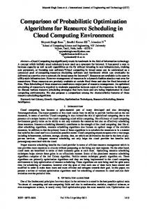
data around the mean value (µ) of this data. It is used to characterize the spread of a distribution of possible outcomes, a probability distribution. This property can be used both to describe the known variability of factors that influence a system (product or process), and as a measure of performance variability, and thus reliability, robustness, or simply quality. A more recent measure of quality is sigma level. Performance variation can be characterized as a number of standard deviations from the mean performance, as shown in Figure 1, to define the sigma level of a product or process. The areas under the normal distribution in Figure 1 associated with each sigma level relate directly to the probability of performance falling in that particular range (for example, ±1σ is equivalent to a probability of 0.683). These probabilities are displayed in Table 1 as percent variation (equivalent to reliability values) and number of defective parts per million parts.

Lower Spec Limit

-6σ

-5σ

-4σ

-3σ

-2σ

design of acceptable quality? Traditionally, if ±3σ worth of performance variation was identified to lie within the set specification limits this was viewed as acceptable variation; in this case, 99.73% of the variation is within specification limits, or the probability of meeting the requirements defined by these limits is 99.73%. In engineering terms, this probability was deemed acceptable. More recently, however, the 3σ quality level has been viewed as insufficient quality, initially from a manufacturing perspective, and then extended into an engineering design perspective. Motorola, in defining “six sigma quality”,7 translated the sigma quality level to the number of defective parts per million (ppm) parts being manufactured. In this case, as can be seen in Table 1, ±3σ corresponds to 2700 ppm defective. This number was deemed unacceptable. Furthermore, Motorola and others observed that even at some observed variation level, mean performance could not be maintained over time. If a part is to be manufactured to some nominal specification, plus/minus some specification limits, the mean performance will change and thus the distribution will shift. A good example of this is tool wear. If a process is set up to manufacture a part to a nominal dimension of 10 in. with a tolerance of ±0.10 in., even if the process meets this nominal dimension on average, the cutting tool will wear with time, and the average part dimension will shift, say to 10.05 in. This will cause the distribution of performance variation to shift, while the specification limits remain fixed, and thus the area of the distribution outside one of the specification limits will increase. This shift was observed by Motorola and others to be approximately 1.5σ, and was used to define “long term sigma quality” as opposed to “short term sigma quality”. This explains the last column in Table 1. While the defects per million for short term correspond directly to the percent variation for a given sigma level associated with the standard normal distribution, the defects per million for long term correspond to a 1.5σ shift in the mean. In this case, 3σ quality leads to 66,803 defects per million, which is certainly unacceptable. Consequently, Motorola defined a quality goal of ±6σ, and “six sigma quality” came to define the desired level of acceptable performance variation. With this quality goal, the defects per million, as shown in Table 1, is 0.002 for short term quality, and 3.4 for long term quality – both acceptable quality levels. The focus on achieving six sigma quality is commonly referred to as Design for Six Sigma (DFSS). In a probabilistic engineering design context, DFSS can be implemented by incorporating the “minimize performance variation” goal of robust design, qualified by the constraints of reliability, by striving to maintain

Upper Spec Limit

-1σ

µ

+1σ +2σ

+3σ +4σ +5σ +6σ

Figure 1 Normal Distribution, 3-σ Design Table 1

Sigma Level as Percent Variation and Defects per Million

Sigma Percent Defects/million Defects/million Level Variation (short term) (long term) ±1σ 68.26 317,400 697,700 ±2σ 95.46 45,400 308,733 ±3σ 99.73 2,700 66,803 ±4σ 99.9937 63 6,200 ±5σ 99.999943 0.57 233 ±6σ 99.9999998 0.002 3.4 Quality can be measured using any of the variability metrics in Table 1 – “sigma level”, percent variation or probability/reliability, or number of defects per million parts (a manufacturing “mass production” measure) – by comparing the associated performance specification limits and the measured performance variation. In Figure 1, the lower and upper specification limits that define the desired performance range are shown to coincide with ±3σ from the mean. The design associated with this level of performance variance would be considered a “3σ” design. Is this

4 American Institute of Aeronautics and Astronautics

Here X includes input parameters which may be design variables, random variables, or both. Both input and output constraints are formulated to include mean performance and a desired “sigma level”, or number of standard deviations within specification limits:

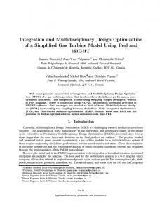
six-sigma (µ±6σ) performance variation within the defined acceptable limits, as illustrated in Figure 2. In Figures 2a and 2b, the mean, µ, and lower specification limit (LSL) and upper specification limit (USL) on performance variation are held fixed. Figure 2a represents the 3σ design of Figure 1; ±3σ worth of performance variation is within the defined specification limits. In order to achieve a 6σ design, one for which the probability that the performance will remain within the set limits is essentially 100%, the performance variation must be reduced (reduced σy), as shown in Figure 2b. An approach for DFSS, or more specifically for optimizing for six sigma quality, incorporating the measures of quality discussed in this section, is detailed in the next section.

-6σy

+6σy

LSL

-3σy

USL

µy

+3σy

(a) 3-σ Design

LSL,USL: Lower, Upper Specification Limits

-6σy

+6σy

LSL

USL

-3σy

µy +3σ

[2]

µy + nσy ≤ Upper Specification Limit

[3]

The robust design objective for this formulation, including “mean on target” and “minimize variation” robust design goals, is generally formulated as follows: l w 1 F = ∑  i µ Yi - M i s i =1   1i

(

)

2

+

w 2i s 2i

 σ Y2i  

[4]

where w1i and w2i are the weights and s1i and s2i are the scale factors for the “mean on target” and “minimize variation” objective components respectively for performance response i, Mi is the target for performance response i, and l is the number of performance responses included in the objective. For the case in which the mean performance is to be minimized or maximized, rather than directed towards a target, the objective formulation of Eqn. 4 can be modified as shown in Eqn. 5, where the first term is positive when the response mean is to be minimized, and negative when the response mean is to be maximized.∗

y

(b) 6-σ Design

Figure 2 Design for Six Sigma

3 APPROACH: PROBABILISTIC MULTIDISCIPLINARY DESIGN OPTIMIZATION EMPLOYING KRIGING Designing for both performance and quality requires a performance model, some understanding of uncertainty for definition of factors that lead to performance variation, a method to measure design quality (to quantify the measure discussed in the previous section), and a strategy for choosing new designs. In this section, a six sigma based probabilistic optimization strategy is presented that combines all of these necessary elements. Implementation of such a strategy for complex multidisciplinary design optimization problems, however, can be extremely computationally expensive. Consequently, kriging, an approximation strategy, is implemented within this probabilistic optimization strategy. An overview of kriging is also provided in this section.

l   w1 w2 F = ∑  ( + / − ) i µYi + i σY2i  s1i s 2i i =1   

[5]

To implement this six sigma based probabilistic optimization formulation, to calculate the robust objective value and quality with respect to constraints (sigma level or reliability), the mean and standard deviation or variance must be estimated for all outputs during optimization. The methods and tools developed for structural reliability analysis and robust design facilitate this estimation. Three classes of methods are used with this formulation: 1. 2. 3.

3.1 Six Sigma Based Probabilistic Optimization Formulation The six sigma based probabilistic design optimization formulation is given as follows: Find the set of design variables X that: Minimizes: F(µy(X),σy(X)) Subject to: gi(µy(X),σy(X)) ≤ 0 XL + nσx ≤ µx ≤ XU- nσx

µy − nσy ≥ Lower Specification Limit

Monte Carlo Simulation • Simple Random Sampling21 • Descriptive Sampling22 Design of Experiments23 Sensitivity Based Estimation • First Order Taylor’s Expansion24 • Second Order Taylor’s Expansion25

Monte Carlo Simulation (MCS) Monte Carlo simulation techniques are implemented by randomly simulating a design or process, given the ∗

[1]

NOTE: Limitations are known to exist with weighted sum type objective functions when generating Pareto sets20; development of alternate formulations is a topic of current research.

5 American Institute of Aeronautics and Astronautics

fewer sample points are necessary for statistical estimates when compared to simple random sampling.

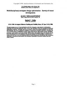
stochastic properties of one or more random variables, with a focus on characterizing the statistical nature (mean, variance, range, distribution type, etc.) of the responses (outputs) of interest.21 Monte Carlo methods have long been recognized as the most exact method for all calculations that require knowledge of the probability distribution of responses of uncertain systems to uncertain inputs. To implement a Monte Carlo simulation, a defined number of system simulations to be analyzed are generated by sampling values of random variables (uncertain inputs), following the probabilistic distributions and associated properties defined for each. Several sampling techniques exist for simulating a population; two techniques are discussed here: simple random sampling,21 the tradition approach to Monte Carlo, and descriptive sampling,22 a more efficient variance reduction technique. These two techniques are compared in Figure 3. With simple random sampling, the traditional MCS approach shown in Figure 3a, sample points are generated randomly from each distribution, as its name implies. Sufficient sample points (often tens of thousands) must be taken to ensure the probability distributions are fully sampled.

Design of Experiments (DOE) A second approach for estimating performance variability due to uncertain design parameters is through more structured sampling, using a designed experiment, a common tool for robust design analysis. In DOE, a design matrix is constructed, in a systematic fashion, that specifies the values for the design parameters (uncertain parameters in this context) for each sampled point, or experiment. A number of experimental design techniques exist for efficiently sampling values of design parameters; for more details on experimental design techniques, see Ref. 23. With DOE, potential values for uncertain design parameters are not defined through probability distributions, but rather are defined by a range (low and high values), a nominal baseline plus/minus some delta or percent, or through specified values, or levels. In this case each run in the designed experiment is a combination of the defined levels of each parameter. Consequently, this approach represents a higher level of uncertainty in uncertain design parameters, with expected ranges rather than specific distributions. The computational cost of implementing DOE depends on the particular experiment design chosen and the levels of the uncertain parameters, but is generally significantly less than that of Monte Carlo simulation. However, the estimates may not be as accurate. This method is recommended when distributions are not known, and can also be used when uncertain parameters are known to vary uniformly.

x2

x2

fX2(x2)

fX2(x2)

x1

x1 fX1(x1)

(a) Simple Random

fX1(x1)

Sensitivity Based Variability Estimation A third approach for estimating performance variability is a sensitivity-based approach, based on Taylor’s series expansions. In this approach, rather than sampling across known distributions or ranges for uncertain design parameters, gradients for performance parameters are taken with respect to the uncertain design parameters, and hence the “sensitivity-based” nature of the approach. Generally with this approach the Taylor’s expansion is either first order, neglecting higher order terms, or second order. Obviously there is a tradeoff between expense (number of gradient calculations) and accuracy when choosing to include or neglect the higher order terms. The first order and second order formulations are given as follows. First Order Taylor’s Expansion. Neglecting higher order terms, the Taylor’s series expansion for a performance response, Y, is:

(b) Descriptive

Figure 3 Monte Carlo Sampling Comparison Variance reduction sampling techniques have been developed to reduce the sample size (number of simulations) without sacrificing the quality of the statistical description of the behavior of the system. Descriptive sampling is one such sampling technique. In this technique, the probability distribution of each random variable is divided into subsets of equal probability and the analysis is performed with each subset of each random variable only once (each subset of one random variable is combined with only one subset of each other random variable). This sampling technique is similar to Latin Hypercube experimental design techniques, and is best described through illustration as in Figure 3b for two random variables. Each row and column in the discretized two variable space is sampled only once, in random order. Only seven points/subsets are shown in Figure 3b for clarity in illustration; obviously more points are necessary for acceptable estimation, but often an order of magnitude

Y(x) = y +

6 American Institute of Aeronautics and Astronautics

dY ∆x dx

[6]

The mean of this performance response is then calculated by setting the uncertain design parameters to their mean value, µx:

evaluation. Consequently, this approach is significantly more computationally expensive than the first order Taylor’s expansion, and usually will be more expensive than DOE. For low numbers of uncertain parameters, this approach can still be more efficient than Monte Carlo simulation, but becomes less efficient with increasing n (Monte Carlo simulation is not dependent on the number of parameters). For efficiency in implementing the second order Taylor’s expansion approach, the cross terms of Eqn. 11 are often ignored, and only pure second order terms are included (diagonal terms). The number of necessary evaluations is then reduced to 2n+1. The second order Taylor’s expansion is recommended when curvature exists and the number of uncertain parameters is not excessive. Any of the sampling methods summarized in this section can be used to estimate performance variability. These estimates are then used within the six sigma probabilistic optimization formulation to improve design quality. As previously discussed, the combination of one of these sampling methods with an optimization procedure, however, may not be computationally feasible for complex multidisciplinary design problems. For this reason, the generation of approximate/surrogate models may be necessary to replace complex analysis codes and allow efficient probabilistic exploration and optimization. Kriging, described next, is implemented here for this purpose.

[7]

µY = Y ( µx )

and the standard deviation of Y(x) is given by: 2

 ∂Y  2 σ Y = ∑   (σ xi ) i =1  ∂xi  n

[8]

where σxi is the standard deviation of the ith parameter and n is the number of uncertain parameters. For more details on this approach for variability estimation for robust design purposes, see Ref. 24. Since first order derivatives of responses with respect to random variables are needed in Eqn. 8, and the mean value point is needed in Eqn. 7, the first order Taylor’s expansion estimates require n+1 analyses for evaluation. Consequently, this approach is significantly more efficient than Monte Carlo simulation, and often more efficient than DOE while including distribution properties. However, the approach loses accuracy when responses are not close to linear in the region being sampled. This method is therefore recommended when responses are known to be linear or close to linear, and also when computational cost is high and rough estimates are acceptable. Second Order Taylor’s Expansion. Adding the second order terms, the Taylor’s series expansion for a performance response, Y, is: Y(x) = y +

dY 1 d 2Y ∆x + ∆x T ∆x dx 2 dx 2

3.2 Kriging Approximation Models Originating in geostatistics,18 kriging models have found much success in approximating deterministic computer simulations.14,26 A kriging model is a combination of a polynomial model plus departures of the form:

[9]

The mean of this performance response is then obtained by taking the expectation of both sides of the expansion: µY = Y ( µ x ) +

1 n d 2Y 2 ∑ σx 2 i dxi 2 i

y(x) = f(x) + Z(x)

where y(x) is the unknown function of interest, f(x) is a known (usually polynomial) function of x, and Z(x) is the realization of a stochastic process with mean zero, variance σ2, and non-zero covariance. The f(x) term in Eqn. 12 provides a “global” model of the design space and is similar to the polynomial model in a response surface. In this work, we take f(x) to be a constant term based on previous studies.15,16 While f(x) “globally” approximates the design space, Z(x) creates “localized” deviations so that the kriging model interpolates the ns sampled data points; however, non-interpolative kriging models can also be created to smooth noisy data.17,27 The covariance matrix of Z(x) is:

[10]

and the standard deviation of Y(x) is given by: σY =

2

2

 ∂Y  1 n n  ∂ 2Y   (σ xi ) 2 + ∑∑   (σ xi ) 2 (σ x j ) 2 [11] ∑ 2 i j  ∂xi ∂x j  i =1  ∂xi  n

[12]

where σxi is the standard deviation of the ith parameter and σxj is the standard deviation of the jth parameter. For more details on this approach for variability estimation and its use for robust design, see Ref. 25. Since second order derivatives of responses, including crossed terms, with respect to random variables are needed in Eqn. 11, and the mean value point is needed in Eqn. 10, the second order Taylor’s expansion estimates require (n+1)(n+2)/2 analyses for

Cov[Z(xi),Z(xj)] = σ2 R([R(xi,xj)]

7 American Institute of Aeronautics and Astronautics

[13]

In Eq. 13, R is the correlation matrix, and R(xi,xj) is the correlation function between any two of the ns sampled data points xi and xj. R is a (ns x ns) symmetric matrix with ones along the diagonal. The correlation function R(xi,xj) is specified by the user, and a variety of correlation functions exist.28-30 In this work, we utilize the popular Gaussian correlation function: 2

R(x i , x j ) = exp[− ∑k dv=1 θ k x ik − x jk ] n

algorithm to perform this optimization. During this fit optimization, the condition number of the correlation matrix is monitored and the optimizer is directed away from areas that lead to ill-conditioning to ensure a wellconditioned kriging model. Booker33 discusses other methods for preserving well-conditioned kriging models. 4 EXAMPLE: CONCEPTUAL MULTIDISCIPLINARY SHIP DESIGN In this section the six sigma based probabilistic optimization strategy presented in the previous section is implemented, employing kriging approximation models for efficient probabilistic optimization. The example problem investigated is the multidisciplinary conceptual design of an oil tanker ship.34 The disciplines involved in the conceptual ship design analysis, shown in Figure 4, include: propulsion, structures, hydrodynamics, cost, and return-oninvestment (ROI). Six design variables are included in this problem:

[14]

where ndv is the number of design variables, θk are the unknown correlation parameters used to fit the model, and xki and xkj are the kth components of sample points xi and xj. In some cases using a single correlation parameter gives sufficiently good results;26,31,32 however, we use a different θ for each design variable to maximize the flexibility of the approximation. Predicted estimates, yˆ (x), of the response y(x) at untried values of x are computed using: yˆ = βˆ + r T (x )R −1 (y − fβˆ )

[15]

1. 2. 3. 4. 5. 6.

where y is the column vector of length ns which contains the sample values of the response, and f is a column vector of length ns which is filled with ones when f(x) is taken as a constant. The correlation vector, rT(x), between an untried x and the sampled data points {x1, ..., xns} is given by: rT(x) = [R(x,x1), R(x,x2), ..., R(x,xns)]T.

hull thickness deck thickness ship length deck height fuel weight installed engine horsepower

[16]

ˆ Meanwhile, the estimate for β is given by:

Propulsion

T −1 −1 T −1 βˆ = (f R f) f R y

Structures

[17]

Hydrodynamics

and the estimate of the variance, σˆ 2, of the sample data, denoted as y, from the underlying global model (not the variance in the observed data itself) is given by: 2 σˆ =

(y − f βˆ ) T R −1 (y − fβˆ )

Cost ROI

Figure 4 Disciplines for Conceptual Ship Design

[18]

ns

The optimization formulation for this conceptual ship design problem, including a single objective and five constraints, is stated as follows:

ˆ β

where f(x) is assumed to be the constant . The maximum likelihood estimates (i.e., “best guesses”) for the θk used to fit the model are found by maximizing: max θ > 0, θ ∈ ℜ

− n

[ns ln(σˆ 2 ) + ln | R |] 2

Maximize: ROI Subject to: Range ≥ 10,000 Nm Displacement Weight ≤ 2*108 lbs. Maximum bending stress ≤ 30 ksi Maximum shear stress ≤ 30 ksi Stability factor ≤ 0.0

[19]

where σˆ 2 and |R| are both functions of θ. While any values for the θk create an interpolative kriging model, the “best” kriging model is found by solving this kdimensional unconstrained non-linear optimization problem. Currently, we are using a simulated annealing

To convert this deterministic optimization formulation to a probabilistic problem, to support both probabilistic analysis of identified solutions and

8 American Institute of Aeronautics and Astronautics

probabilistic optimization to improve design quality, six random variables are added to the problem as defined in Table 2. All six random variables are assumed to vary normally, with standard deviations equal to 3% of the mean value. Sea water properties are taken at approximately 50 °F.

stress in some regions and significantly under-predicts in the high stress area. The over-prediction may be tolerable in deterministic optimization since feasible values exist, but the best ROI value may not be identified. For the probabilistic optimization, however, over-prediction has a larger impact. Since the probability of violating the stress constraint is being evaluated, over-predicting stress will over-predict the probability of failure, which could make it more difficult to identify quality solutions with respect to all constraints. Under-predicting stress could lead to higher failure probability than predicted.

Table 2 Conceptual Ship Design Random Variables Random Variable 1. propeller efficiency 2. drivetrain efficiency 3. density of steel, lb/ft3 4. density of sea water, slug/ft3 5. viscosity of sea water, ft2/sec 6. fuel cost, $/gallon

µ 0.60 0.90 489.0 1.992 1.56e-5 1.0

σ 0.018 0.027 14.67 0.0598 4.67e-7 0.03

Deterministic optimization is first performed for this problem to ensure that feasible designs exist before implementing the more expensive probabilistic optimization. The actual analysis codes are used for this deterministic optimization, which requires 198 analyses (198 executions of the analysis codes for all 5 disciplines). A sequential quadratic programming (SQP) based algorithm is employed for this deterministic optimization; results are given in Table 3. A probabilistic analysis of the deterministic solution yields a sigma level of 0.64 for this design, a reliability of less than 50%, due to both stress constraints being active. This probabilistic analysis result justifies the application of probabilistic optimization to improved the quality of the design and reduce the probability of violating the stress constraints. To facilitate probabilistic optimization, kriging approximation models are constructed for each of the six responses (the ROI objective and five constraint responses) to replace the codes associated with the five ship design disciplines. To construct these models, a Latin hypercube DOE with 200 sampling points is executed with the actual analysis codes. As an example of the models produced, bending stress is plotted versus ship length and deck thickness in Figure 5. Note that this is only a 2-design variable slice through a six design variable space, and these plots are very simple for this problem. However, the accuracy of the kriging model is clear in these plots. In Figure 5a, the kriging model is plotted along with the actual data. The kriging model captures the shape of the actual data nearly exactly. Note that the kriging model plot in Figure 5a is generated by executing the kriging model over a different set of points than those used to fit the model; since a kriging model will interpolate the original data points, predictions at those point will not truly represent the shape of the model for untried points. A quadratic response surface fit is shown for comparison in Figure 5b. The response surface over-predicts the bending

(a) Kriging Model

(b) Quadratic Response Surface

Figure 5 Bending Stress vs. Ship Length and Deck Thickness The probabilistic optimization formulation for this problem expands the objective to include minimization of the ROI variation and adjusts the constraints to seek solutions that remain six standard deviations within the original constraint boundaries. This probabilistic optimization formulation is given as follows: Minimize:

-µROI+σROI

Subject to: µRange-6σRange ≥ 10,000 Nm µDisplacement Weight + 6σDisplacement Weight ≤ 2*108 lbs. µMax Bending Stress + 6σMax Bending Stress ≤ 30 ksi µMax Shear Stress + 6σMax Shear Stress ≤ 30 ksi µStability factor + 6σStability factor ≤ 0.0

9 American Institute of Aeronautics and Astronautics

Probabilistic optimization results for the conceptual ship design problem are given in the last column of Table 3. A genetic algorithm is employed with the probabilistic formulation above, operating on the kriging models constructed, and the first order Taylor’s sampling method is employed for variability estimation for a total of 1512 approximate analyses. The quality of the ship design is increased over 8σ for all constraints, essentially 100% reliability (note that the probability of failure for >8σ is beyond the limits of double precision calculations). In reaching this quality level, the necessary tradeoff is realized in the reduction of mean ROI by 7.5%; however, for the probabilistic solution, the standard deviation of ROI is reduced by 10.7%, making this a more robust design. These probabilistic optimization results obtained using the kriging approximation models are verified by performing a robust analysis at this solution point using the actual analysis codes; the difference between the code-based and kriging-based results are too small to display in Table 3. Table 3

REFERENCES [1] Thanedar, P. B. and Kodiyalam, S., 1991, “Structural Optimization using Probabilistic Constraints”, 32nd AIAA/ASME/ACE/AHS/ASC Structures, Structural Dynamics and Materials Conference, pp. 205-212, AIAA-91-0922-CP. [2] Chen, X., Hasselman, T.K., and Neill, D.J., 1997, “Reliability Based Structural Design Optimization for Practical Applications,” 38th AIAA/ASME/ ASCE/AHS/ASC, Structures, Structural Dynamics and Materials Conference, Kissimmee, FL, pp. 2724-2732. Paper No. AIAA-97-1403. [3] Xiao, Q., Sues, R. H., and Rhodes, G. S., 1999, “Multi-Disciplinary Wing Shape Optimization with Uncertain Parameters,” 40th AIAA/ASME/ASCE/ AHS/ASC Structures, Structural Dynamics, and Materials Conference, St. Louis, MO, pp. 30053014. Paper No. AIAA-99-1601. [4] Koch, P. N., Wujek, B., and Golovidov, O., 2000, “A Multi-Stage, Parallel Implementation of Probabilistic Design Optimization in an MDO AIAA/USAF/NASA/ISSMO Framework,” 8th Symposium on Multidisciplinary Analysis and Optimization, Long Beach, CA., AIAA-2000-4805. [5] Melchers, R.E., 1999, Structural Reliability: Analysis and Prediction, Second Edition, Ellis Horwood Series in Civil Engineering, John Wiley & Sons, New York. [6] Ross, P.J., 1996, Taguchi Techniques for Quality Engineering, Second Edition, McGraw-Hill, New York. [7] Harry, M.J., 1997, The Nature of Six Sigma Quality, Motorola University Press, Shaumburg, IL. [8] Pande, P.S., Neuman, R.P., and Cavanagh, R.R., 2000, The Six Sigma Way: How GE, Motorola, and Other Top Companies are Honing Their Performance, McGraw-Hill, New York.

Conceptual Ship Design Results

ROI Range Displacement. Weight Bending Stress Shear Stress Stability

This probabilistic multidisciplinary optimization with kriging models is demonstrated for the conceptual design of an oil tanker ship; a “six sigma” solution is presented and verified. For this simple example problem, probabilistic optimization with the actual codes, starting from the deterministic optimization solution, requires over 3000 system analyses using the most efficient sampling method, with variability estimates based on a first order Taylor’s expansion. The expense of probabilistic optimization increases rapidly with more accurate sampling methods and with problem size and complexity. The use of good approximation models is essential. The example provided here is only an illustration of the concepts and applicability. Further investigation and development is underway with more complex multidisciplinary problems.

Deterministic Optimization Solution 0.307 std. dev. = 0.00941 >8σ 100% >8σ 100% 0.643 σ 47.98% 0.644 σ 48.02% >8 100%

Probabilistic Optimization with Kriging Models 0.274 std. dev. = 0.00840 >8σ 100% >8σ 100% >8σ 100% >8σ 100% >8σ 100%

5 SUMMARY AND CLOSING REMARKS In this paper an approach to probabilistic design optimization is presented that combines methods from reliability-based design and robust design with the more recent six sigma concepts. The six sigma based probabilistic optimization formulation presented supports modeling of variability in all aspects of the formulation: bounds on random design variable, tolerance variable variation to be optimized, output constraint reliability, and a robust objective formulation. All of these elements combine to facilitate the measurement and improvement of the “sigma level” quality of a design. In this paper, kriging approximation models are employed within the six sigma based probabilistic optimization approach to provide a strategy for applying these methods to complex multidisciplinary design problems. 10

American Institute of Aeronautics and Astronautics

[9] Koch, P., N., 2002, “Probabilistic Design: Optimizing for Six Sigma Quality,” 43rd AIAA/ASME/ASCE/AHS Structures, Structural Dynamics, and Materials Conference, 4th AIAA Non-Deterministic Approaches Forum, Denver, Colorado, AIAA-2002-1471. [10] Koch, P, N. and Cofer, J. I., 2002, “SimulationBased Design in the Face of Uncertainty,” JANNAF Interagency Propulsion Committee, 2nd Modeling and Simulation Subcommittee, Destin, FL. [11] Myers, R.H.; Montgomery, D.C., 1995, Response Surface Methodology: Process and Product Optimization Using Designed Experiments, John Wiley & Sons, New York. [12] Koch, P. N., Simpson, T. W., Allen, J. K., and Mistree, F., 1998, "Statistical Approximations for Multidisciplinary Design Optimization: The Problem of Size," AIAA Journal of Aircraft, Vol. 36, No. 1, pp.275-286. [13] Koch, P. N., Mavris, D., and Mistree, F., 2000, "Partitioned, Multi-Level Response Surfaces for Modeling Complex Systems," AIAA Journal, Vol. 38, No. 5, pp. 875-881. [14] Simpson, T. W., Peplinski, J. D., Koch, P. N., and Allen, J. K., 2001, "Metamodels for ComputerBased Engineering Design: Survey and Recommendations," Journal of Engineering with Computers, Vol. 17, No.2, pp. 129-150. [15] Simpson, T. W., Mauery, T. M., Korte, J. J. and Mistree, F., 2001, “Kriging Models for Global Approximation in Simulation-Based Multidisciplinary Design Optimization”, AIAA Journal, Vol. 39, No. 12, pp. 2233-2241. [16] Jin, R., Chen, W. and Simpson, T. W., 2002, “Comparative Studies of Metamodeling Techniques under Multiple Modeling Criteria”, Journal of Structural and Multidisciplinary Optimization, Vol. 23, No. 1, pp. 1-13. [17] Cressie, N. A. C., 1993, Statistics for Spatial Data, Revised Edition, John Wiley & Sons, New York. [18] Matheron, G., 1963, “Principles of Geostatistics,” Economic Geology, Vol. 58, pp. 1246-1266. [19] Koch, P. N., Evans, J. P., and Powell, D., 2002, “Interdigitation for Effective Design Space Exploration using iSIGHT,” Journal of Structural and Multidisciplinary Optimization, Vol. 23, No. 2, pp. 111-126. [20] Athan, T.W. and Papalambros, P.Y., 1996, “A Note on Weighted Criteria Methods for Compromise Solutions in Multi-Objective Optimization,” Engineering Optimization, Vol. 27, No. 2, pp. 155-176. [21] Hammersley, J.M., and Handscomb, D.C., 1964, Monte Carlo Methods, Chapman and Hall, London.

[22] Saliby, E., 1990, “Descriptive Sampling: A Better Approach to Monte Carlo Simulation”, J. Opl. Res. Soc., Vol. 41, No. 12, pp. 1133-1142. [23] Montgomery, D. C. 1996, Design and Analysis of Experiments, New York: John Wiley & Sons. [24] Chen, W., Allen, J. K., Tsui, K.-L., and Mistree, F., 1996, “A Procedure for Robust Design: Minimizing Variations Caused by Noise Factors and Control Factors,” ASME Journal of Mechanical Design, Vol. 118, No. 4, pp. 478-485. [25] Hsieh, C-C., and Oh, K. P., 1992, “MARS: a computer-based method for achieving robust systems,” FISITA Conference, The Integration of Design and Manufacture, Vol. 1, pp. 115-120 [26] Sacks, J., Welch, W. J., Mitchell, T. J. and Wynn, H. P., 1989, "Design and Analysis of Computer Experiments," Statistical Science, Vol. 4, No. 4, pp. 409-435. [27] Montès, P., 1994, "Smoothing Noisy Data by Kriging with Nugget Effects," Wavelets, Images and Surface Fitting (Laurent, P. J., Le Méhauté, A., et al., eds.), A.K. Peters, Wellesley, MA, pp. 371378. [28] Koehler, J. R. and Owen, A. B., 1996, "Computer Experiments," Handbook of Statistics (Ghosh, S. and Rao, C. R., eds.), Elsevier Science, New York, pp. 261-308. [29] Mitchell, T. J. and Morris, M. D., 1992, "Bayesian Design and Analysis of Computer Experiments: Two Examples," Statistica Sinica, Vol. 2, pp. 359379. [30] Sacks, J., Schiller, S. B. and Welch, W. J., 1989, "Designs for Computer Experiments," Technometrics, Vol. 31, No. 1, pp. 41-47. [31] Booker, A. J., Dennis, J. E., Jr., Frank, P. D., Serafini, D. B., Torczon, V. and Trosset, M. W., "A Rigorous Framework for Optimization of Expensive Functions by Surrogates," Structural Optimization, Vol. 17, No. 1, 1999, pp. 1-13. [32] Osio, I. G. and Amon, C. H., "An Engineering Design Methodology with Multistage Bayesian Surrogates and Optimal Sampling," Research in Engineering Design, Vol. 8, No. 4, 1996, pp. 189206. [33] Booker, A., "Well-Conditioned Kriging Models for Optimization of Computer Simulations," Technical Document Series, M&CT-TECH-00-002, Phantom Works, Mathematics and Computing Technology, The Boeing Company, Seattle, WA, 2000. [34] Kodiyalam, S.; Su Lin, J.; Wujek, B.A. 1998: Design of Experiments Based Response Surface Models for Design Optimization. 39th AIAA/ASME/ASCE/AHS/ASC Structures, Structural Dynamics and Materials Conference, Long Beach, CA, AIAA-1998-2030, pp. 27182727. 11

American Institute of Aeronautics and Astronautics