Aug 22, 2006 - Bhai, Zaid, Zubair, Pasha, Asif, Hassan and Saif for their much ...... [17] Markus A. Dangl, Zhenning Shi, Mark C. Reed, and Jürgen Lindner.
Factor Graphs and MCMC Approaches to Iterative Equalization of Nonlinear Dispersive Channels by
Faisal M. Kashif Submitted to the Department of Electrical Engineering and Computer Science in partial fulfillment of the requirements for the degree of Master of Science in Electrical Engineering and Computer Science at the MASSACHUSETTS INSTITUTE OF TECHNOLOGY Aug 2006 c Massachusetts Institute of Technology 2006. All rights reserved. �
Author . . . . . . . . . . . . . . . . . . . . . . . . . . . . . . . . . . . . . . . . . . . . . . . . . . . . . . . . . . . . . . Department of Electrical Engineering and Computer Science Aug 22, 2006 Certified by . . . . . . . . . . . . . . . . . . . . . . . . . . . . . . . . . . . . . . . . . . . . . . . . . . . . . . . . . . Moe Z. Win Associate Professor Thesis Supervisor
Accepted by . . . . . . . . . . . . . . . . . . . . . . . . . . . . . . . . . . . . . . . . . . . . . . . . . . . . . . . . . Arthur C. Smith Chairman, Department Committee on Graduate Students
2
To my parents, and To the people who could not survive the 1947 migration.
3
4
Factor Graphs and MCMC Approaches to Iterative Equalization of Nonlinear Dispersive Channels by Faisal M. Kashif Submitted to the Department of Electrical Engineering and Computer Science on Aug 22, 2006, in partial fulfillment of the requirements for the degree of Master of Science in Electrical Engineering and Computer Science
Abstract In this work, equalization for nonlinear dispersive channels is considered. Nonlinear communication channels can lead to significant degradations when nonlinearities are not taken into account at either the receiver or the transmitter. In many cases, the nonlinearity of the channel precludes the use of spectrally efficient signaling schemes to achieve high data-rates and the bandwidth efficiency. Satellite channel is a typical case of nonlinear channel that needs to be used efficiently. We develop two novel equalization strategies for a general class of nonlinear channels. Both strategies are based on iterating between decoding and equalization, termed as iterative equalization. The first strategy is a factor graph based equalizer that converts the nonlinear channel equalization problem into forward-backward algorithm on hidden Markov model (HMM). The equalizer is implemented via the sum-product algorithm on the factor graph representation of the channel and receiver blocks. The second equalization strategy is based on Markov chain Monte Carlo (MCMC) methods. We typecast the problem of executing forward-backward algorithm on HMM into an MCMC domain problem and develop four different types of MCMC equalizers. These solutions have different performance and magnitudes of complexity. For the purpose of performance analysis of our equalizers, simulation results were obtained for two different scenarios: Quadrature Phase Shift Keying (QPSK) and 16Quadrature Amplitude Modulation (QAM). Significant performance gain compared to the linear equalizer is reported for both factor graph and MCMC strategies. We also present a detailed performance and complexity analysis of the equalizers. Both equalization strategies require knowledge of the channel. In many practical situations, the channel has to be estimated. To this end, we consider two scenarios: first, when the channel model/structure is known and second, when there is no information regarding the channel structure. In the first case, we derive a maximumlikelihood (ML) channel estimator for a Volterra structure based nonlinear channel and evaluate the estimator’s performance bounds. We also explore the optimal pilot design and present simulation results. In the second scenario, when no model for the 5
channel is available, we propose use of the de Bruijn sequence as the pilot to perform the ML estimation of the channel function. While developing MCMC iterative equalization, we set up the problem such that MCMC technique efficiently solves the inference for an HMM based system with reduced computational cost. In general, inference on an HMM based system has a complexity that is exponential in the size of the state-space of the system, however our MCMC based solution has a linear complexity. This aspect of our strategy can be generalized to other engineering applications involving HMM structure. Thesis Supervisor: Moe Z. Win Title: Associate Professor
6
Acknowledgments I would like to thank Prof. Moe Win for his time, guidance and support throughout this research. He showed me the way to this research topic and it has introduced me to so many new and exciting problems. I would have not been able to complete this research without his advice and constant mentoring. I am greatly indebted to Henk Wymeersch who took so much time on daily basis to discuss my research problems and encouraged me to take up the immediate next challenge. He has been a source of inspiration and learning for me. He has helped me throughout this work in various aspects and has read and corrected my numerous write-ups that are generally so hard to understand for anyone else. I am grateful to Dr Sohail Naqvi for his instrumental guidance, mentorship and teaching. It goes back to my Signal & Systems days, and encompasses all important stages of my career. I would have not made thus far without you, sir! I am also extremely fortunate to have been in contact with Dr Syed Ismail Shah. He has taught me, advised me and cared for me like a friend. He has supported me when I needed the most. I want to take this opportunity to express my sense of gratitude to you, sir. Many thanks to Dr Jamil Ahmad for his positive presence and influence on my plans to come to MIT. Syed Wajih Umar, he has been such a big help, guide, support and friend that I have started taking it for granted. Thank you, Wajih! Life in Boston would have been so unmanagebale otherwise. Abdurrehman, Aspen and little Zaineb have provided me love, in addition to the food and support provided by their parents: Aamnia Bhabi and Wajih. Thankoooo! Special thanks to my PP, Syed Hassan Saud, for his unique friendship and support at all times. He has helped me keep my focus. I also thank Jahanzeb Latif for his tremendous role and then companionship all the way. I cannot ever pay it back. Thanks to Safdar Ali Khan for all the discussions and ‘being with’. This definitely made decisions easier. I would have run into a different “Markov chain” of life, otherwise. Thanks to Umar Iqbal and Yasir Javed, for their “breezy” influence; I 7
have often tried to copy you. Umar also wrote a letter on my behalf and made me send that; it moved things for me to join here. Many thanks to Abdelhak for his pleasant companionship and kind gestures at the moments of need. Among the friends around the campus, I am thankful to Rehan Bhai, Zaid, Zubair, Pasha, Asif, Hassan and Saif for their much needed company and tolerance. Special thanks to Zubair Anwar for providing his computer access for running simulations. Thanks to Sadaf and Bushra Bhabi for providing so-great home-food at numerous occasions. It just makes me feel at home. Thanks to Ahmed Bhai for his care. I am thankful to Imran, Omar and Mobien for their consistent companionship and care even when there are long distances between Helsinki, London and Boston. How can I not mention Tariq, who is at Amherst these days but has responded to every call of mine and visited me. In addition to that you and your family have played a tremendous role in all this, and I am deeply grateful for that. I cannot express due thanks to the one who trusted me and played a pivotal role in setting off my career 10 years back. There is a long list of such people from my school-days, but this one role supercedes. And then those who make me feel I exist! I am wholeheartedly thankful to my parents, brothers and sisters for their love, care and cooperation throughout my life. It was impossible to plan this journey without the confidence that you gave me. Special thanks to Bhayya, Dr Khalid Mahmood, who spent sleepless nights so that I could get started with my career. Of course, I owe an unpayable debt to my parents, who loved me enough to let me go! This work was supported, in part, by the National Reconnaissance Office, the Charles Stark Draper Laboratory Robust Distributed Sensor Networks Program, the Office of Naval Research Young Investigator Award N00014-03-1-0489, and the National Science Foundation under Grant ANI-0335256.
8
Contents Contents
9
List of Figures
13
List of Tables
17
1 Introduction
19
1.1
Motivation . . . . . . . . . . . . . . . . . . . . . . . . . . . . . . . . .
20
1.2
Nonlinear Channel Models . . . . . . . . . . . . . . . . . . . . . . . .
21
1.3
Previous Work
. . . . . . . . . . . . . . . . . . . . . . . . . . . . . .
21
1.4
Our Approach . . . . . . . . . . . . . . . . . . . . . . . . . . . . . . .
23
1.5
Organization of Thesis . . . . . . . . . . . . . . . . . . . . . . . . . .
23
1.6
Notation . . . . . . . . . . . . . . . . . . . . . . . . . . . . . . . . . .
24
2 System and Channel Model
25
2.1
Overview . . . . . . . . . . . . . . . . . . . . . . . . . . . . . . . . . .
25
2.2
System and Channel Model Details . . . . . . . . . . . . . . . . . . .
26
2.3
Concluding Remarks . . . . . . . . . . . . . . . . . . . . . . . . . . .
28
3 Channel Estimation
29
3.1
Overview . . . . . . . . . . . . . . . . . . . . . . . . . . . . . . . . . .
29
3.2
Structure-based Channel Estimation . . . . . . . . . . . . . . . . . .
30
3.2.1
Channel Structure . . . . . . . . . . . . . . . . . . . . . . . .
31
3.2.2
Channel Estimator and Performance Bounds . . . . . . . . . .
31
9
3.2.3 3.3
3.4
Results and Discussion . . . . . . . . . . . . . . . . . . . . . .
34
Structure-less Channel Identification . . . . . . . . . . . . . . . . . .
41
3.3.1
Identifying g(·) . . . . . . . . . . . . . . . . . . . . . . . . . .
41
3.3.2
Using de Bruijn Sequence as Pilot . . . . . . . . . . . . . . . .
42
Concluding Remarks . . . . . . . . . . . . . . . . . . . . . . . . . . .
43
4 Mathematical Tools 4.1
4.2
4.3
45
Factor Graphs and the Sum-Product Algorithm . . . . . . . . . . . .
45
4.1.1
Factor Graphs . . . . . . . . . . . . . . . . . . . . . . . . . . .
45
4.1.2
Sum-Product Algoithm . . . . . . . . . . . . . . . . . . . . . .
47
Markov Chain Monte Carlo Methods . . . . . . . . . . . . . . . . . .
48
4.2.1
Monte Carlo (MC) Integration . . . . . . . . . . . . . . . . . .
49
4.2.2
Weighted Importance Sampling . . . . . . . . . . . . . . . . .
49
4.2.3
MCMC
. . . . . . . . . . . . . . . . . . . . . . . . . . . . . .
50
Concluding Remarks . . . . . . . . . . . . . . . . . . . . . . . . . . .
51
5 Iterative Equalization for Nonlinear Channels
53
5.1
Iterative Equalization . . . . . . . . . . . . . . . . . . . . . . . . . . .
53
5.2
Factor Graph Equalizer for Nonlinear Channels . . . . . . . . . . . .
58
5.3
MCMC Equalizer for Nonlinear Channels . . . . . . . . . . . . . . . .
61
5.3.1
MCMC-I . . . . . . . . . . . . . . . . . . . . . . . . . . . . . .
64
5.3.2
MCMC-II . . . . . . . . . . . . . . . . . . . . . . . . . . . . .
65
5.3.3
MCMC-III . . . . . . . . . . . . . . . . . . . . . . . . . . . . .
66
5.3.4
MCMC-IV . . . . . . . . . . . . . . . . . . . . . . . . . . . . .
66
5.3.5
Remarks on Implementation . . . . . . . . . . . . . . . . . . .
66
Concluding Remarks . . . . . . . . . . . . . . . . . . . . . . . . . . .
67
5.4
6 Results and Discussion
69
6.1
Description of the Simulation Setup . . . . . . . . . . . . . . . . . . .
69
6.2
Performance of the Factor Graph Equalizer . . . . . . . . . . . . . . .
70
6.3
Performance of the MCMC Equalizer . . . . . . . . . . . . . . . . . .
72
10
6.4
Computational Complexity and Storage Requirements . . . . . . . . .
74
7 Conclusions
77
8 Appendix
79
8.1
Volterra Series based Nonlinear Channel Model . . . . . . . . . . . .
79
8.1.1
Implementation . . . . . . . . . . . . . . . . . . . . . . . . . .
79
8.1.2
Matrix Representation of the Volterra Structure . . . . . . . .
81
Bibliography
83
11
12
List of Figures
2-1 The System Model: a block of bits b is coded into c and mapped to symbols block x. Transmitter applies pulse-shape and the continuoustime channel output is converted into discrete-time channel observations r. Equalizer and decoder jointly recover the transmitted bit sequence. . . . . . . . . . . . . . . . . . . . . . . . . . . . . . . . . . . .
27
2-2 The Channel Model: xk are the transmitted symbols, L is the discrete channel memory and g(·) represents the equivalent channel function. nk represents circularly symmetric Gaussian noise. . . . . . . . . . . .
27
3-1 Block diagram view of the receiver where channel estimation block is included to provide equalizer with the estimated channel function gˆ(·).
30
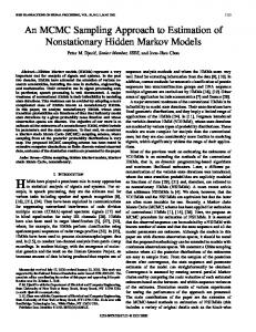
3-2 Approximate optimal performance bounds and the actual MSE of the estimator are shown at different SNR values, with P = 20 in QPSK. .
36
3-3 QPSK: approximate distribution of the MCRB of the estimator for randomly chosen pilot sequences (top). The region where distribution is concentrated is zoomed in the lower panel. Minimum MCRB for the case of optimal pilot sequence is indicated by line with solid dot, and the mean MCRB is indicated by line with + sign. . . . . . . . . . . . � �−1 3-4 The structure of matrix AH A (in figure window (a)) and AH A
37
(in figure window (b)) for the approximate optimal pilot sequence with P = 20, in QPSK. AH A appears almost a scaled identity matrix as expected for the optimal performance. . . . . . . . . . . . . . . . . . 13
37
3-5 Approximate optimal performance bounds and the actual MSE of the estimator are shown at different SNR values, with P = 20 in 16-QAM.
38
3-6 16-QAM: approximate distribution of the MCRB of the estimator for randomly chosen pilot sequences (top). The region where distribution is concentrated is zoomed in the lower panel. Minimum MCRB for the case of optimal pilot sequence is indicated by line with solid dot, and the mean MCRB is indicated by line with + sign. . . . . . . . . . . . � �−1 3-7 The structure of matrix AH A (in figure window (a)) and AH A
39
(in figure window (b)) for the approximate optimal pilot sequence with P = 20, in 16-QAM. AH A appears almost a scaled identity matrix as expected for the optimal performance. . . . . . . . . . . . . . . . . .
39
3-8 Channel estimator’s MCRB as a function of number of pilot symbols, P at a fixed SNR. This plot corresponds to QPSK transmission at SNR=7 dB. . . . . . . . . . . . . . . . . . . . . . . . . . . . . . . . .
40
4-1 An example of a factor graph. A distribution p(x1 , x2 , x3 , x4 , x5 ) represented as the product of three functions p1 , p2 and p3 , each of which depends on only a subset of variables in p. Variables are represented by edges and the functions by nodes. Some of the messages are shown for description. Once p2 has messages from x2 and x3 , it can compute � message to x4 , i.e., µp2→x4 = ∼{x4 } p2 (x2 , x3 , x4 )µx2 →p2 µx3 →p2 . . . . .
46
5-1 Factor graph of the complete iterative receiver. The scheduling of message computation is indicated by the labelled arrows. The first level nodes are fk = p(rk |yk ), that compute messages based on given channel observations r. The last step is the computation of messages over the bk -edges, in the direction indicated by arrow F. In the figure, ˜ � K − 1. . . . . . . . . . . . . . . . . . . . . . . . . . . . . . . . . K
56
5-2 Iterative Equalization of Nonlinear Channel: r is the received block of channel observations. The equalizer and decoder work iteratively to recover b, the sequence of transmitted bits. . . . . . . . . . . . . . . . 14
58
5-3 Factor graph for the Nonlinear Channel/Equalizer based on the HMM description of the channel. The sum-product algorithm on this graph computes the probability distributions for each xk . The result is therefore equivalent to the forward-backward algorithm. First and last state edges are connected with square blocks to indicate that their messages may be known through initialization. . . . . . . . . . . . . . . . . . .
60
5-4 Sum-product algorithm for the upward messages from the kth node in Fig. 5-3 . . . . . . . . . . . . . . . . . . . . . . . . . . . . . . . . . .
60
6-1 QPSK: Iteration 1, 2 and 3 of factor graph equalizer for the nonlinear channel (indicated as FG-NLIE) are compared with the equalizer that only takes care of the linear ISI. Matched filter (MF) bound and the genie bound are also plotted for the sake of reference. . . . . . . . . .
71
6-2 16-QAM: Iteration 1, 2 and 3 of Factor graph equalizer for the nonlinear channel (indicated as FG-NLIE) are shown. Matched filter (MF) bound and the genie bound are also plotted for the sake of reference. The linear channel equalizer is not shown due to poor performance. .
71
6-3 MCMC equalizers for QPSK: BEP vs SNR performance of all the four methods is compared with the factor graph equalizer (indicated as FG). 73 6-4 MCMC equalizers for 16-QAM: BEP vs SNR performance of MCMCIII and MCMC-IV is compared with the factor graph equalizer (indicated as FG). Results are shown for different number of parallel Gibbs samplers (GS). . . . . . . . . . . . . . . . . . . . . . . . . . . . . . .
74
6-5 Computational complexity vs performance trade-off in MCMC methods: reducing S2 from 2 to 1 decreases the performance by about 0.7 to 1 dB at high SNR’s. Decreasing S2 to 0 results in almost 2 dB drop in performance. Results presented in this figure correspond to MCMC-IV. Similar trends were observed for MCMC-I and MCMC-III. 15
75
6-6 Comparison of the computational cost of equalizers for the nonlinear channel in 16-QAM. MCMC methods have the same parameters and performance as described in the previous section. . . . . . . . . . . .
76
8-1 Nth order Volterra based representation of the noiseless channel function. 81
16
List of Tables 6.1
Comparison of the Computational and Storage Requirements of the factor graph (FG) and MCMC equalizers . . . . . . . . . . . . . . . .
17
76
18
Chapter 1 Introduction Communication channel has been a topic of great interest to researchers for its various interesting and challenging aspects. Interesting because this adds uncertainty to the communication system and we have to resort to the “guessing game,” also known as probability theory; and challenging because there is always room for making a more “educated guess.” Various physical phenomena that are undesired, and sometimes unaccounted for as well, are trivially lumped into the channel block of the communication system, that is connected to the transmitter at one end and the receiver on the other. Through the enormous amount of attention given to communication systems, we today know a large number of different communication channels and are able to communicate through them, with various efficiency levels. The efficient use of channel requires maximizing the information transfer for a certain power and bandwidth resources with minimum error. The maximum capacities and error-performance of various channels have been figured out and coding and signaling schemes have been developed to make transceivers that operate close to these capacity and performance limits. However, this is not finished yet. Nonlinear type of communication channel is an example of one such area where we still need to make progress towards the optimal performance. In this chapter, we introduce the problem and provide a background of the efforts towards the solution. We briefly bring up the salient features of our approach. 19
1.1
Motivation
The satellite channel is limited in terms of both power and bandwidth. Therefore, it is critical to use this channel efficiently and achieve high data-rates by employing spectrally efficient signaling/modulation schemes [30]. However, the satellite channel is a nonlinear dispersive channel with both amplitude and phase distortion [1, 9, 15, 31, 55], limiting the use of spectrally efficient schemes such as quadrature-amplitude modulation (QAM) and degrading the performance of other schemes, such as phaseshift keying (PSK) [7]. Hence, the system operates at a reduced data-rate and yields degraded performance [6, 14, 30, 31]. The fundamental cause of nonlinearity in the satellite path is the high power amplifier (HPA) at the transmitter which, for reasons of power efficiency, is operated near its saturation point. The problem is further exacerbated owing to the nonlinearity being frequency-dependent [9, 55].
On the whole, nonlinear channels can be categorized into the following three types, based on the source: transmitter-based nonlinearity, inherent physical channel nonlinearity, receiver-based nonlinearity. A nonlinear communication channel can be due to any one or more of these sources. Apart from the satellite channel, nonlinear channels also appear in other scenarios such as microwave communication [28], optical fiber communication [60, 61], magnetic recording [40, 46], and optical recording [13] channels. Additionally, higher order intermodulation products in certain communication lines and some receiver components such as rectifiers, clippers, envelope detectors also introduce nonlinearity [38]. In some cases the nonlinearity can be safely ignored (e.g., the nonlinearity of some detection algorithms and devices such as square-law detector, and synchronization blocks). However, other types of nonlinearity have severe effect on the performance and efficiency of the communication system. Thus, there is a large set of communication scenarios that are affected by nonlinearity whose overall effect is that conventional receivers perform poorly. 20
1.2
Nonlinear Channel Models
Various models for the nonlinear channel have been presented [6, 31, 55]. Modeling efforts have traditionally been made from different perspectives: a faithful model of nonlinearity may be in a form that is not easy to simulate a communication system; a simulation model may not be the basis for the development of a receiver; and a simple signal-processing blocks based model may not be accurate enough. Some of the representative works on the nonlinear channel models can be found in [6,9,31,55].
1.3
Previous Work
To mitigate the adverse effects of nonlinear channels, various approaches have been proposed in technical literature [5, 32, 49, 52]. The work can be grouped into two major categories: transmitter-based solutions [4, 15, 16, 32, 33], and receiver-based solutions [5, 32, 49, 64]. In the former category, the most important are data predistortion and analog pre-distortion. A data pre-distorter modifies the transmitter constellation to take into account the effects of the nonlinear channel [10, 33, 34, 43]. Analog pre-distortion (also called signal pre-distortion), aims at reducing the nonlinear distortion of the transmitter amplifier by driving it with an input signal such that the desired signal is transmitted. Transmitter-based schemes suffer from three problems: a) they can not be applied to legacy systems, b) they require knowledge of the nonlinear channel, c) they are typically focused on minimizing the spectral regrowth and maintaining the signal integrity, whereas it is hard to devise transmitterbased schemes to directly minimize the bit-error probability (BEP) of the system [32]. Consequently, receiver-based solutions have to be sought. Receiver-based approaches to cope with nonlinear channels rely mainly on equalization. Several kinds of equalizers for nonlinear channels have been presented in literature: a Volterra series based equalization for the case of 16-QAM in a nonlinear channel was discussed in [5]. Maximum-likelihood sequence detection (MLSD) based nonlinear channel equalizer was presented in [7, 27, 44, 64]. Inter-symbol interference 21
(ISI) cancellation strategies were discussed in [57], and later extended to trellis-coded systems in [56]. Equalization for coded systems was also considered in [22] and [62]. Among the recent developments, a blind equalization solution based on �-algorithms for binary inputs was presented in [3]. A fuzzy adaptive equalizer has been considered in [65] and adaptive equalizers using artificial neural networks have been presented in [35, 49, 50]. Equalization techniques specific to nonlinear magnetic recording channels have been discussed in [40, 46, 48]. A common weakness in the majority of these equalization techniques is that the equalizer operates independently of the decoder. These techniques either work with uncoded systems, or if a coded system is considered, the decoder and equalizer are designed as independent blocks. With the introduction of turbo-codes [8], it has been recognized that equalization and decoding can be jointly designed to provide substantial performance gains. The basic idea of turbo (or iterative) equalization is to iterate between equalization and decoding stages and was presented for a frequencyselective linear channel in [24, 39]. An insightful tutorial on the topic can be found in [36]. In the context of nonlinear channels, however, this idea has not yet been fully explored. A few efforts in this regard are the work of [11, 29, 59]. Equalization combined with trellis-coded modulation (TCM) and turbo-TCM was discussed in [29] where a gain of 1 dB compared with the conventional separate equalization was reported for 16-QAM TCM at BEP of 10−3. Simulation results for iterative equalization-decoding for a Volterra based nonlinear channel were presented in [59]. An ISI canceller based turbo equalization strategy for 16-QAM was simulated in [11], using the Saleh model of memoryless nonlinear channel [55] along with transmit and receive filters. Recently, [47] has employed remedial techniques both at the transmitter and the receiver using non-uniform 16-QAM together with turbo codes for the nonlinear channels, and simulations results are given for the Saleh model [55] for memoryless nonlinearity and root-Nyquist transmit and receive filters. So far, the works on iterative equalization for nonlinear channels are incomplete as the approach towards developing solutions has been ad-hoc. Moreover, they have focused on a specific type of nonlinearity. 22
1.4
Our Approach
In this work, we develop two novel equalization strategies for a general class of nonlinear channels. Our strategies are derived in a systematic (as opposed to an ad-hoc) way, based on two mathematically rigorous methods: factor graphs and Markov chain Monte Carlo (MCMC) methods. This leads to what we name as the factor graph equalizers and MCMC equalizers, respectively. In the second category, four types of MCMC equalizers are described. Through simulations, we show that both the approaches provide significant performance gains compared to the linear equalizer. Even the cases where linear equalizer may completely fail, iterative equalizers provide excellent performance. We also quantify the computational complexity of the different equalization strategies. Both equalization strategies require knowledge of the channel. In many practical situations, the channel has to be estimated. To this end, we consider two scenarios: first, when the channel model/structure is known and second, when there is no information regarding the channel structure. In the first case, we derive a maximumlikelihood (ML) channel estimator for a Volterra structure based nonlinear channel and evaluate the estimator’s performance bounds. We also explore the optimal pilot design and present simulation results. In the second scenario, when no model for the channel is available, we propose use of the de Bruijn sequence as the pilot to perform the ML estimation of the channel function.
1.5
Organization of Thesis
The thesis is organized as follows: Chapter 2 describes the system and channel model that is used to develop iterative equalization solutions in the rest of the work. Chapter 3 covers the topic of channel estimation where we first derive an estimator for the nonlinear channel with a known model and analyze estimator’s performance; in the second part, we discuss the case where no channel model information is available. In Chapter 4, we give an overview of factor graphs and MCMC methods in a general 23
setting. In Chapter 5, we provide the solutions to the nonlinear channel problem; the main idea of nonlinear iterative equalization is explained , followed by the derivation of the factor graph and MCMC equalizers. Chapter 6 provides the detailed results, performance analysis and a detailed view of the computational and storage requirements of the equalizers developed in this work. Finally, Chapter 7 concludes the thesis. Appendix provides details about the famous Volterra model for the nonlinear channel that we refer in the channel estimation in Chapter 3, and also in the simulations for the performance analysis of our equalization algorithms.
1.6
Notation
The following notation is used in this work: f (x) ∝ g(x) when f (x) = Ag(x) for some constant A. Vectors (row-vectors) are denoted in bold. In the vector indices, i : j is used to indicate from start index to end index, with i and j as the start and end indices respectively. E {·} denotes the expectation operator. We denote the probability distribution pX1 ,X2 ,...,Xn (x1 , x2 , . . . , xn ) simply as p(x1 , x2 , . . . , xn ) for brevity. This is also the treatment with conditional distributions, e.g., pX1 |X2 (x1 |x2 ) is denoted as p(x1 |x2 ). Along the same lines, a variable is simply denoted with small letters, e.g, xk even when it refers to a random variable. This simplifies the reading as most of this thesis talks about random variables and probability distribution functions, except at a few instances which should be clear from the context. The term function has been used in the general sense, specifically in the context of factor graphs, but invariably in this work, the function at hand is a probability distribution function.
24
Chapter 2
System and Channel Model
2.1
Overview
The goal of any digital communication system is to successfully transfer an information bit sequence from the transmitter location to the receiver location. Depending on the particular application and the setup requirements, various choices of information representation, encryption, coding and signaling schemes are available. Also, the medium that is used for transmission and related equipment impacts the overall design as well as performance of the communication system. Our goal is to develop generic equalization strategies for solving the nonlinear dispersive channel problem, and we take a fairly general communication system by keeping the other blocks of the communication system as general as possible. This chapter provides the details of the system and the channel model adopted for the equalizer design in later chapters. Both the system and channel models are flexible so that the equalizers designed based on these models remain applicable to any general scenario of nonlinear dispersion. 25
2.2
System and Channel Model Details
We consider a coded transmission scheme
1
where the encoder function X (·) maps a
block b of Nb information bits to Nc coded bits: c = X (b). Based on the selected modulation scheme, the mapper function φ(·) maps the block of coded bits to a block of K symbols, x = [x0 , x1 , . . . , xK−1], such that xk ∈ Ω, where Ω is the constellation of size M = |Ω|. Finally, the block of symbols, x, is transmitted through the channel. The baseband-equivalent continuous-time transmitted signal s(t) is given by � � K−1 xk p(t − kT ), s(t) = Es
(2.1)
k=0
where Es is the energy per symbol, and p(t) is the transmitter pulse (for example, a Nyquist pulse, a root-raised-cosine pulse) with symbol duration T . This signal passes through a nonlinear channel, giving rise to the signal y(t) = C {s(t)}, where C {·} represents the baseband equivalent nonlinear channel. At the receiver, the signal y(t) is corrupted by additive white Gaussian noise (AWGN) process n(t) with power spectral density N0 /2 per real dimension. The received waveform can be written as r(t) = y(t) + n(t).
(2.2)
The complete system model is given in Fig. 2-1. At the receiver, the baseband waveform r(t) is converted into a discrete-time observation r through suitable filtering and digital conversion. Thus, r is the block of K channel observations, r = [r0 , r1 , . . . , rK−1 ]. The overall equivalent discrete-time channel model, shown in Fig. 2-2, is given by: yk = g(xk , xk−1 , . . . , xk−L),
(2.3)
rk = yk + nk ,
(2.4)
1
This is required for the iterative equalization. However, the equalization algorithms are applicable to an uncoded transmission system as well, without benefiting from the gain associated with their iterative processing.
26
Figure 2-1: The System Model: a block of bits b is coded into c and mapped to symbols block x. Transmitter applies pulse-shape and the continuous-time channel output is converted into discrete-time channel observations r. Equalizer and decoder jointly recover the transmitted bit sequence. for k = 0, 1, . . . , K − 1. Here, g(·) is the channel function representing the discretetime equivalent of the nonlinear channel and L is the channel memory. Hence, g(·) nonlinearly combines a block of L+1 symbols, [xk , xk−1 , . . . , xk−L ] to produce yk . The symbols x−1 , x−2 , . . . , x−L are all either 0, or unknown, depending on the specific scenario.
xk
g(xk , xk−1, . . . , xk−L)
rk
yk
nk
Figure 2-2: The Channel Model: xk are the transmitted symbols, L is the discrete channel memory and g(·) represents the equivalent channel function. nk represents circularly symmetric Gaussian noise. The term nk represents the circularly symmetric Gaussian noise, nk ∼ Nc (0, σ 2 ), where σ 2 /2 = N0 /2Es is the variance of real and imaginary noise components. Mathematically,
� � 1 ||n||2 p(n) = exp − 2 πσ 2 σ 27
(2.5)
2.3
Concluding Remarks
In this chapter, we described the overall system model and presented a generic nonlinear channel model that encapsulates a wide class of non-linear (and linear) channels, including the well-known Volterra series based model [7] that has been commonly used to represent the travelling-wave-tube-amplifier (TWTA) in the satellite communication setup. This generic channel model, represented as g(·), forms the basis for development of the equalizers in the later chapters. Chapter 3 briefly discusses the problem of estimating this channel function.
28
Chapter 3 Channel Estimation 3.1
Overview
In the previous chapter, we have introduced the channel function g(·), that encapsulates the nonlinear dispersion: rk = yk + nk ,
(3.1)
yk = g(xk , xk−1 , ...xk−L ).
(3.2)
where xk is the kth transmitted symbol, xk ∈ Ω, L is the channel memory, nk circularly symmetric AWGN with zero mean and variance of σ 2 /2 = N0 /2Es , per real dimension. Most important of all, g(·) is the channel function, and is assumed to be known at the beginning of the receiver operation. However, in practice, g(·) has to be estimated. In this chapter, we consider this channel estimation block. The block diagram of the receiver with channel estimation is shown in Fig. 3-1. We consider two scenarios for the estimation of the nonlinear dispersive channel. The first scenario is when the channel structure is known, such as the Volterra channel model, and we aim at estimating the coefficients of the model. It must be clarified that channel estimation process depends heavily on the choice of channel model/structure, signaling and modulation scheme, as well as the bandwidth and power constraints of the system. In the second scenario we have no information about the channel 29
Figure 3-1: Block diagram view of the receiver where channel estimation block is included to provide equalizer with the estimated channel function gˆ(·). structure. In this case, we suggest an approach to perform channel identification using the de Bruijn sequences [18]. In this chapter, we start by discussing the first approach of estimating the channel coefficients of the Volterra model. We consider data-aided (or pilot-based) channel estimation and develop a Maximum-Likelihood (ML) estimator. We also analyze the performance of the estimator, derive the performance bounds and draw some conclusions regarding the number of pilots and the design of the pilot signal. In the next section, we consider the scenario when no channel model can be assumed and discuss employing the de Bruijn sequences to identify the channel function g(·).
3.2
Structure-based Channel Estimation
The development in this section is general and applicable to any channel structure. However, for the sake of example to clearly articulate the channel estimation process, we consider a Volterra series based expansion for the nonlinear channel. This has the advantage of efficiently capturing the nonlinear behavior and has been very often used to describe the nonlinear systems [7]. However, we want to stress that our receiver designs in the forthcoming chapters will be generic as they do not depend on any particular choice of the channel function. A detailed description of the Volterra series based representation is provided in the Appendix. We assume that the order of the Volterra model and the number of taps are known. Moreover, we consider an 30
independent pilot signal transmission for the purpose of channel estimation before the actual data transmission.
3.2.1
Channel Structure
Let a be the block of P known pilot symbols, transmitted through the channel. We start by writing the channel function relationship based on the Volterra model. The received block r of channel observations can be written as: r = Ah + n,
(3.3)
where h is the vector of Q channel coefficients that need to be estimated, where Q depends on the order N and the memory length L of the Volterra model: Q = �N i 1 The matrix A is P × Q and has a systematic form in terms of the i=1 (L + 1) . pilot symbols a. The general forms of matrix A and the channel coefficients vector h for an Nth order Volterra based channel model with memory L, are specified in Appendix A. Finally, n = [n0 , n1 , . . . , nP −1 ]T , where nk ∼ Nc (0, σ 2 ).
3.2.2
Channel Estimator and Performance Bounds
The Estimator ˆ is given by, Given the received block r, the ML estimator h ˆ = arg max p(r|h). h h∈CQ
(3.4)
Due to the monotonicity of the log function, ˆ = arg max ln p(r|h), h h∈CQ
1 = arg min 2 ||r − Ah||2 , Q σ h∈C � H �−1 H A r. = A A 1
(3.5) (3.6) (3.7)
In some cases, Q may be less, as some of the coefficients can be known to be zeros; for example, in case of pass-band signaling, the Volterra model requires only the odd power terms.
31
The estimator requires the matrix AH A to be invertible, which implies P ≥ Q and a ∈ ΩP selected such that AH A is a well-conditioned matrix.
Performance of the Estimator
It can be easily seen that the estimator is unbiased. Taking expectation over r, � �� �−1 H H ˆ A r , E h =E A A �� � −1 H H A (Ah + n) , =E A A �� � � �−1 H −1 = E AH A AH Ah + AH A A n , �−1 H � A E {n} , = h + AH A = h.
(3.8) (3.9) (3.10) (3.11) (3.12)
Similarly, the covariance matrix of the estimation error is found to be, � ˆ = E (h − h)(h ˆ ˆ H , Var{h − h} − h)
� � H �−1 H �� H �−1 H H A A A n A A A n , =E �−1 H � H � � H �−1 � A E nn A A A , = AH A � �−1 H 2 � �−1 = AH A A σ IA AH A , � �−1 H � H �−1 A A A A , = σ 2 AH A � � −1 . = σ 2 AH A
(3.13) (3.14) (3.15) (3.16) (3.17) (3.18)
Performance Bounds ˆ with the known pilot sequence a, we have actually In the design of estimator h worked with p(r|h; a), where a is a deterministic nuisance parameter. Along the lines suggested in [45], we derive the the Modified Cramer-Rao Bound (MCRB) to benchmark the estimator’s performance. The Fisher Information matrix J is given 32
by [63]: �� �H � ∂ ∂ , J(h) = E ln p(r|h, a) ln p(r|h, a) ∂h ∂h �� �� �H � ∂ ∂ 1 , ||r − Ah||2 ||r − Ah||2 = 4E σ ∂h ∂h ��
=
1 H A A. σ2
(3.19) (3.20) (3.21)
Hence, the MCRB on the estimator of the channel coefficients is given by: MCRB = J−1 (h), � �−1 = σ 2 AH A .
(3.22) (3.23)
ˆ is efficient, as it achieves the MCRB perforFrom (3.18) we see that the estimator h mance.
Optimal Pilot Sequence Design We have evaluated the performance of the estimator for a given pilot sequence a. Now it is of primary interest to find the pilot sequence that has the lowest MCRB, or has the minimum Mean-Squared Error (MSE). This essentially requires the minimization of the trace of MCRB in (3.23). Hence, the optimal pilot sequence of length P is given by: aopt = arg min T a∈ΩP
��
H
A A
�−1 �
.
(3.24)
where T(M) calculates the trace of any matrix M. Let λ1 , λ2 , . . . , λQ be the eigenvalues of AH A, then 1/λ1 , 1/λ2 , . . . , 1/λQ are the �−1 � eigenvalues of AH A . Since the trace of a matrix can be written as the sum of its eigenvalues, T
��
H
A A
�−1 �
33
Q � 1 . = λ i i=1
(3.25)
Substituting (3.25) in (3.24) yields,
aopt = arg min a∈ΩP
Q � 1 . λ i i=1
(3.26)
� �−1 is minimized. That is, select a ∈ ΩP such that the sum of the eigenvalues of AH A �Q 1 Observe that i=1 λi is dominated by 1/λmin , where λmin = min(λ1 , λ2 , ..., λQ ), is the smallest eigenvalue of AH A. A near-optimal sequence may be found as: aopt ≈ arg max λmin . a∈ΩP
(3.27)
Overall, this optimization process depends on the selected constellation, signal power, length of the pilot sequence and the channel, which dictates the structure of the matrix A. Depending on a particular situation, it may be analytically tractable to find the optimal sequence using (3.27). Otherwise, a brute-force search for the optimal sequence becomes cumbersome for large values of P and the constellation size.
3.2.3
Results and Discussion
Simulation Setup In this channel estimation exercise, we consider the following Volterra channel function: yk = (0.780855 + j0.413469)xk + (0.040323 − j0.000640)xk−1 + (−0.015361 − j0.008961)xk−2 +(−0.04 − j0.009)xk xk x∗k + (−0.035 + j0.035)xk xk x∗k−1 + (0.039 + j0.022)xk xk x∗k−2 +(−0.001 − j0.017)xk−1xk−1 x∗k + (0.018 − j0.018)xk−2 xk−2 x∗k . where xk is the kth complex symbol transmitted either from QPSK or 16-QAM constellations, and ∗ denotes the complex conjugate operation. These channel coefficients are unknown to the receiver and we apply the ML estimator described above to estimate them. To set up the estimator, we first form the matrix A and the vector h as 34
(3.28)
specified in the Appendix. a 0 a1 A= .. . aP −1
a−1 a−2
a20 a∗0
a20 a∗−1
a20 a∗−2
a2−1 a∗0
a2−2 a∗0
a0 .. .
a21 a∗1
a21 a∗0
a21 a∗−1
a20 a∗1
a2−1 a∗1
a−1 .. .. . .
.. .
.. .
.. .
.. .
aP −2 aP −3 a2P −1 a∗P −1 a2P −1 a∗P −2 a2P −1 a∗P −3 a2P −2 a∗P −1 a2P −3 a∗P −1
(3.29)
where ai are pilot symbols from the block a. Correspondingly, take h = [h1 , h2 , ...hQ ]T , comprising of only the non-zero coefficients in (3.28). In this reduced form, there are eight unknown coefficients for the estimator, i.e., Q = 8. We employ the estimator for two different transmission schemes: QPSK and 16-QAM. Note that for QPSK, xk xk x∗k = Es xk so that in (3.28) we can merge the first and the fourth term, reducing Q to 7. A needs to be modified accordingly.
Results for QPSK To find the optimal pilot sequence for a given P , we can use a computer program to numerically solve (3.26) for small values of P and small constellations. However, for relatively large P this brute-force search becomes impractical; for example, even at P = 20 in QPSK, it requires a search on 240 sequences. We modified the search for an optimal pilot sequence by sampling uniformly in ΩP and choosing the best sample. With P = 20, and 10000 uniformly distributed samples, the best sequence is selected as the “approximate optimal” sequence. This approximate optimal pilot sequence yields an MCRB as shown in Fig. 3-2 for different values of SNR. An actual estimator for based on this sequence was constructed and its MSE was calculated through Monte Carlo simulation. Fig. 3-2 shows that the MSE for this estimator is the same as the MCRB. The average MCRB for the randomly chosen pilot sequences is also shown in the figure2 . Note that the approximate optimal sequence results in a 3 dB gain as compared to the average performance. 2
In the performance MCRB actually refers to the trace of the MCRB matrix defined �� analysis, �−1 � . previously, i.e., σ 2 T AH A
35
0
10
MCRB (approx. optimal) Estimator’s sample MSE Average MCRB
−1
MSE
10
−2
10
−3
10
0
2
4
6
8
10 SNR [dB]
12
14
16
18
20
Figure 3-2: Approximate optimal performance bounds and the actual MSE of the estimator are shown at different SNR values, with P = 20 in QPSK. The distribution of the MCRB is shown in Fig. 3-3. This gives us an idea of the whole performance range, as well as the probability of randomly picking a close to optimal pilot sequences, without performing the optimization described in the last section.
� �−1 as they “control” We also want to get insight into the matrix AH A or AH A
the performance of the estimator. For the approximate optimal pilot sequence, Fig. 34-(a) shows AH A. It is strictly diagonally-dominant, almost an identity matrix, and the diagonal entries are proportional to the number of pilot symbols and their energy. The inverse of this matrix is shown in Fig. 3-4-(b). Intuitively, this makes sense as �−1 � the optimal sequence minimizes the trace of AH A .
Results for 16-QAM The same steps as above were performed for the case of 16-QAM with P = 20. The search for the optimal sequences yielded an approximate optimal sequence whose MCRB and an actual MSE are shown for various SNR values in Fig. 3-5. It also shows the average MCRB for the randomly chosen sequences. To get an idea of the 36
approx. Distribution of MCRB
0.028 0.024 0.020 0.016 0.012 0.008
0.004 0
0
2
0
0.5
4
6 8 MCRB for random pilot sequences
10
12
14
approx. Distribution of MCRB
0.028 0.024 0.020 0.016 0.012 0.008 0.004 0
1
1.5 2 2.5 MCRB for random pilot sequences
3
3.5
Figure 3-3: QPSK: approximate distribution of the MCRB of the estimator for randomly chosen pilot sequences (top). The region where distribution is concentrated is zoomed in the lower panel. Minimum MCRB for the case of optimal pilot sequence is indicated by line with solid dot, and the mean MCRB is indicated by line with + sign.
H
A A
(AH A)−1
0.06
20 18
0.05
16 0.04
14 12
0.03
10 0.02
8 6
0.01
4 0 7
2 7
0 7
6
6 6
1
3
2
2
2
5 4
3
3
3
6 4
4
4
7
5
5 5
1
2 1
(a)
1
(b)
� �−1 Figure 3-4: The structure of matrix AH A (in figure window (a)) and AH A (in figure window (b)) for the approximate optimal pilot sequence with P = 20, in QPSK. AH A appears almost a scaled identity matrix as expected for the optimal performance.
37
0
10
MCRB (approx. optimal) Estimator’s sample MSE Average MCRB
−1
MSE
10
−2
10
−3
10
5
10
15 SNR [dB]
20
25
Figure 3-5: Approximate optimal performance bounds and the actual MSE of the estimator are shown at different SNR values, with P = 20 in 16-QAM. distribution of MCRB for various the pilot sequences, Fig. 3-6 shows a histogram of the MCRB. It is clear that the MCRB in case of 16-QAM is more spread out than in QPSK. In other words, the chance of randomly selecting a close to optimal pilot sequence is smaller and the cost of sub-optimal selection is also higher for 16-QAM than in QPSK. This phenomenon is also observed through the matrices AH A and � H �−1 A A shown in Fig. 3-7-(a) and Fig. 3-7-(b), respectively. Unlike the case of QPSK, these matrices have a more sparse structure. This is also due to the fact that 16-QAM have symbols of three different energy levels whereas for QPSK all the symbols are of the same energy.
Estimation Performance vs Number of Pilot Symbols It is of interest to evaluate the performance of the ML estimator against the number of pilot symbols. Fig. 3-8 shows the approximate optimal MCRB for QPSK for various number of pilot symbols. Approximate optimal sequences were found through the same approach as explained above. As expected, the figure shows that increasing the number of pilot symbols provides better estimation performance. The performance 38
approx. Distribution of MCRB
0.006 0.005 0.004 0.003 0.002 0.001
approx. Distribution of MCRB
0
0
2
1
1.5
4
6 8 MCRB for random pilot sequences
10
12
14
0.005 0.004 0.003 0.002 0.001 0 2
2.5 3 3.5 MCRB for random pilot sequences
4
4.5
5
Figure 3-6: 16-QAM: approximate distribution of the MCRB of the estimator for randomly chosen pilot sequences (top). The region where distribution is concentrated is zoomed in the lower panel. Minimum MCRB for the case of optimal pilot sequence is indicated by line with solid dot, and the mean MCRB is indicated by line with + sign.
H
H
(A A)
−1
(A A)
50
0.7 0.6
40 0.5
30
0.4 0.3
20
0.2
10 0.1
0 8
0 8
8
6
7
4
5 4
2
3 0
6
4
5 2
8
6
7 6
4
2
3 0
1
(a)
2 1
(b)
� �−1 (in Figure 3-7: The structure of matrix AH A (in figure window (a)) and AH A figure window (b)) for the approximate optimal pilot sequence with P = 20, in 16QAM. AH A appears almost a scaled identity matrix as expected for the optimal performance.
39
gain increases rapidly in the beginning, around the minimum number of pilot symbols required for the estimator (i.e., P ≥ Q). From the slope of the MCRB, we observe that we require approximately 75 pilot symbols to reduce the MCRB by an order of magnitude.
0
MCRB
10
−1
10
−2
10
10
15
20
25 No. of pilot symbols
30
35
40
Figure 3-8: Channel estimator’s MCRB as a function of number of pilot symbols, P at a fixed SNR. This plot corresponds to QPSK transmission at SNR=7 dB.
Conclusions A few straightforward conclusions can be drawn from the observations above: the structure of the matrix A suggests that diagonal elements of AH A are proportional to number of pilot symbols P , and the energy of the symbols, Es . For most cases, the matrix is diagonally dominant, positive definite. Therefore, increasing P and the signal power will decrease the MSE of the estimator. In case of 16-QAM, the matrix is not diagonal and the search for optimal pilot sequence is more critical, as well as challenging. 40
3.3
Structure-less Channel Identification
If no channel structure information is available, the estimation process cannot be carried out as discussed in the previous section. In this case, we propose to use a pilot sequence such that all the combinations a ∈ ΩL+1 are passed through the channel and the corresponding channel output for each a is recorded in a table. This table is an identification of the channel function g(·). The accuracy of the identification is inversely related to the channel noise variance and can be increased by repeating the pilot sequence. The important parameter in this scheme is the design of such a pilot sequence. We now explain this channel identification idea in detail and suggest a suitable sequence.
3.3.1
Identifying g(·)
Let us first explain this simple basic idea. In (3.2), let ak represent the sequence [xk , xk−1 , ...xk−L ], of L + 1 symbols xk ∈ Ω. This sequence ak is transmitted through an unknown channel g(·), and results in the noiseless channel output yk = g(ak ). The channel function can be identified by transmitting all the |Ω|L+1 combinations of a and recording the corresponding channel outputs in a list. This list completely characterizes the g(·). For k = 0, 1, . . . , 2L+1 − 1, yk = g(ak ).
(3.30)
For example, in case of binary signaling, Ω = {0, 1} and L = 1, the list has only four combinations: a0 = [0, 0], a1 = [0, 1], a2 = [1, 1] and a3 = [1, 0]. The corresponding channel outputs completely specify channel function g(·). This discussion has ignored the noise term as in our model (3.2), therefore the accuracy of the channel estimate will depend on the amount of noise. In general, applying the ML principle, we find the following channel identification for k = 0, 1, . . . , 2L+1 −1: yˆk = rk = g(ak ) + nk . 41
(3.31)
We see that the variance of the estimate is equal to the noise variance σ 2 . For practical consideration, the identification process need to be carried out at high SNR values. Alternatively, variance reduction techniques are required to improve the accuracy of yˆk in (3.31). A straightforward approach is to transmit each ak multiple times, say (i)
N, and then combining the observations rk as: N 1 � (i) r , yˆk = N i=1 k
= g(ak ) +
N 1 � (i) n , N i=1 k
(3.32) (3.33)
√ so that the variance of the estimator becomes σ 2 / N . Therefore, the accuracy of the estimated channel function is inversely related to the noise variance and directly related to the square root of repetition in pilot transmission.
3.3.2
Using de Bruijn Sequence as Pilot
The interesting part in this channel identification is to design a sequence that has the desired properties as required above but takes the smallest transmission time/resources. This requires the shortest pilot sequence that spans all the |Ω|L+1 combinations. The de Bruijn sequence is known to have this property [18, 54], and is defined as follows: A de Bruijn sequence, denoted as B(k, n), is a k-ary cyclic sequence where each subsequence of length n appears only once, and k is the size of the alphabet of letters in the sequence. The key point is that B(k, n) contains all the combinations of length n. Therefore, for the pilot sequence, we take a de Bruijn sequence d with k = |Ω| and n = L + 1 as it spans all the desired a in its sub-sequences of length L+1. As desired, the length of this de Bruijn sequence is |Ω|L+1 and each channel output corresponds to a distinct a. Thus, de Bruijn sequence is the most efficient pilot sequence for structure-less channel identification purposes. Detailed study of the properties of de Bruijn sequences can be found in [18,54]. A relevant point is that there are generally more than one distinct de Bruijn sequences; 42
number of distinct de Bruijn sequences is related to the constellation size and the memory as:
(|Ω|!)|Ω|L . |Ω|L+1
For the channel identification, we need to construct only one de
Bruijn sequence for each Ω and L. This can be achieved by the algorithm specified in [58], or can be directly obtained in commercial software.
3.4
Concluding Remarks
In this chapter, we covered the topic of channel estimation using the pilot transmission and derived its performance bounds. We considered both structured channel estimation (based on the Volterra models) and structure-less channel estimation (when no model for the channel is available, other than the memory constraint). For structured channel estimation, we have derived the ML estimator, and showed that it achieves the MCRB. Simulation results were used to obtain approximate optimal pilot sequence and to gain an insight into the number of pilots for a desirable estimation performance. In the cases where no model information is available, we discussed using de Bruijn sequences as pilot sequence and perform the channel identification. These sequences result in the shortest possible pilots.
43
44
Chapter 4 Mathematical Tools To develop iterative equalizer for nonlinear channel, we employ two mathematically rigorous approaches: factor graphs and Markov chain Monte Carlo methods. Although these techniques have been used in other problems previously [17, 19, 20, 26, 66,68,69], they are relatively new and we feel the need to describe them clearly before using them in the equalizer design in the next chapter. This chapter first provides an overview of the factor graphs and the associated sum-product algorithm. Later it describes the Markov chain Montre Carlo methods.
4.1 4.1.1
Factor Graphs and the Sum-Product Algorithm Factor Graphs
Factor graphs provide a canonical representation for functions that can be written as a product of two or more factors. They offer a convenient way to compute the marginals associated with those functions. Their natural applications are in estimation, detection, and decoding algorithms, for example, maximum a-posteriori (MAP) estimation, because these algorithms involve functions of several variables (e.g., the joint probability density functions) which conveniently break-down into factors (e.g., because of independence of the component variables in the joint density, or into conditional densities) and their marginal computations are required for the optimization 45
problem (e.g., to find minimum or maximum on a particular dimension). Here, we will only describe the basic concepts here. A more detailed study on factor graphs can be found in literature [37, 41, 67]. As mentioned earlier, a factor graph is a graphical representation of a global function of several variables in terms of its factors and their variables. In the graph, edges denote variables and vertices (which we will call nodes) represent the factors/functions. Although factor graphs provide a general tool applicable to a wide range of applications, we only have to deal with the functions which are (scaled) probability distributions. Let p(x1 , x2 , . . . , xn ) be a joint distribution of n variables which can be factored as: p(x1 , x2 , . . . , xn ) =
J �
pj (χj ),
j=1
where J is the number of factors, χj is a subset of {x1 , x2 , . . . , xn }.
p1
µp1 →x2
x2
x1 µx1 →p1
p2
µp2 →x4
p3
x4
x3 µx3 →p2
x5 µp3 →x5
Figure 4-1: An example of a factor graph. A distribution p(x1 , x2 , x3 , x4 , x5 ) represented as the product of three functions p1 , p2 and p3 , each of which depends on only a subset of variables in p. Variables are represented by edges and the functions by nodes. Some of the messages are shown for description. � Once p2 has messages from x2 and x3 , it can compute message to x4 , i.e., µp2 →x4 = ∼{x4 } p2 (x2 , x3 , x4 )µx2 →p2 µx3 →p2 . As an example, Fig. 4-1 shows a factor graph for n = 5 and J = 3: the distribution p(x1 , x2 , x3 , x4 , x5 ) can be factored into p1 (x1 , x2 ), p2 (x2 , x3 , x4 ), and p3 (x4 , x5 ). Edges connected to only a single node (such as x1 in Fig. 4-1) are called half-edges. Similarly, a node connected to only one edge is called a leaf-node. The key advantages of the Factor Graphs are: From the Factor Graph, it becomes 46
easier to arrange the factors of global function for the marginal computation that is a commonly required step in many engineering algorithms.
4.1.2
Sum-Product Algoithm
In many problems, we are interested in the marginal qi (xi ) of variable xi , defined as qi (xi ) =
�
p(x1 , x2 , . . . , xn ),
∼{xi }
where
� ∼{xi }
indicates the sum operation over all the variables except xi . There is
a systematic procedure for marginal computation on factor graphs, called the SumProduct Algorithm. It is a message-passing algorithm, whereby messages are computed in the nodes and passed over the edges of the factor graph. A message over an edge (say xi ) is a probability distribution of that variable. We will denote the message over edge xi to node pj as µxi →pj (xi ). Note that, if xi is a common edge between function nodes pj and pk , then µpj →xi (xi ) is the same as µxi →pk (xi ). The sum-product algorithm operates as follows: • Initialization: From every leaf-node pj incident with edge xi send message µpj →xi (xi ) = pj (xi ). From every half-edge xk incident with node pl send message � µxk →pl (xk ) = 1. µxk →pl (xk ) = c, s.t. • Message Update Rule: At a node pj , an outgoing message to an incident edge xi can be computed if messages from all other edges incident with node pj are available. This outgoing message is computed as: µpj →xi (xi ) = γ
�
pj (χj )
�
µxj →pj (xj ).
(4.1)
xj ∈χj ,xj �=xi
∼{xi }
The constant γ ensures that the output message is a valid probability distrib� ution: xi µpj →xi (xi ) = 1. We repeat this procedure until all the messages on the graph are computed. At the end, there will be two messages on each edge. 47
• Termination: For any variable, say xi , the corresponding marginal is given by: qi (xi ) = Aµxi →pj (xi )µpj →xi (xi ),
(4.2)
where A is a normalization constant and pj is any node incident with edge xi .
The sum-product algorithm can be shown to provide exact marginals on factor graphs without cycles. However, in case a factor graph has cycles, the result obtained by (4.2) should be interpreted as an approximation of the true marginal qi (xi ).
4.2
Markov Chain Monte Carlo Methods
Monte Carlo methods have long been used in other fields of science and engineering, such as physics and chemical engineering [21, 23, 25, 53], but their role in communication systems has been limited to evaluate error-rate performance of a given system. In recent years, however, they have assumed a rather new role in the design of communication receivers [17, 19, 20, 69]. They have been successfully applied to detection and decoding for various communication systems in computationally intensive scenarios [17, 20, 69]. The basic methodology of the Monte Carlo schemes is to change a “combinatorial” problem into a probabilistic one. Then construct the specific “experiment”, run it a large number of times and count the events of interest to approximate desired result, as opposed to performing the actual deterministic or combinatorial calculations which may be too intensive. Monte Carlo methods are used to approximate multi-dimensional problems integrations to avoid a complexity that is exponential in the number of dimensions involved. A subclass of Monte Carlo methods is MCMC methods [12, 21, 25, 42]. We briefly describe these methods here. 48
4.2.1
Monte Carlo (MC) Integration
Let X be a random variable (possibly multi-dimensional) with distribution fX (x) for we wish to compute the expected value of some function h(X): � E {h(X)} =
h(x)fX (x)dx.
(4.3)
Then, Monte Carlo integration will approximate this integral by Ns � ¯h = 1 h(x(n) ), Ns n=1
where
(4.4)
� (n) �Ns x are Ns samples drawn from the distribution fX (x). As Ns → ∞, n=1
a.s. ¯ −→ E {h(X)}. h
The computational gain of using MC method can be realized if we consider x as a � multi-dimensional variable, hence f (x) a multi-dimensional density, so that dx is a multi-dimensional integration. The general procedures of integration have complexity that grows exponentially with the number of dimensions. However, it can be easily observed that the MC based implementation of (4.4) is not affected by the number of dimensions. The above example is related to computing the expectation, or integral of a function of a random variable, however, MC methods can be applied to approximate deterministic integrals as well. Any one of the functions inside integral is chosen as the “target” distribution to generate samples from and then the rest of the computations follow as in (4.4).
4.2.2
Weighted Importance Sampling
A modified form of the above Monte Carlo technique is the weighted importance sampling. The basic idea of weighted importance sampling is to choose an alternate distribution qX (x) (known as the sampling distribution, as opposed to the target distribution fX (x)) to draw samples from, such that a smaller number of samples from qX (x) provide the same convergence in (4.4). However, the computations are 49
then modified as: ¯= h
Ns �
h(x(n) )w(x(n) ),
(4.5)
n=1
where (n)
w(x
fX (x(n) ) qX (x(n) )
) = �N s
fX (x(n) ) n=1 qX (x(n) )
.
(4.6)
In the special case where qX (x) is uniform distribution, this results in ¯= h
4.2.3
�Ns
n=1
h(x(n) )fX (x(n) )
� Ns
(n) ) n=1 fX (x
.
(4.7)
MCMC
We described above a few basic Monte Carlo methods. An important step in all of them is to draw samples from an arbitrary distribution. In general, we need to draw samples from large-dimensional distributions. In this context, various samplegenerating strategies and algorithms have been traditionally used [19, 21, 23, 42, 53]. MCMC is a powerful class of methods in this regard. It involves constructing a Markov process with the transition probability such that its limiting invariant distribution is the required target distribution [12]. The first such method is the Metropolis-Hasting algorithm which involves acceptance-rejection sampling, and it has various modified forms [19]. Gibbs sampling algorithm is another MCMC method, initially proposed by Geman and Geman (1984) and then extended by Tanner and Wong (1987) and Gelfand and Smith (1990) [12]. In our equalizer design, we will employ the Gibbs sampler. Therefore, we describe this method below. 4.2.3.1
The Gibbs Sampler
Given a multi-dimensional target distribution p(x) as well as the fully conditional distributions for each component, the Gibbs sampler operates as follows: � (n) (n) (n) • Goal: Draw Ns samples x = x0 , . . . , xD−1 for n = 1, 2, . . . , Ns from a D-dimensional distribution p(x), using fully conditional densities: p(xi |x0 , x1 , . . . , xi−1 , xi+1 , . . . , xD−1 ), ∀i. 50
• Initialization:
� (−B) (−B) (−B) Start n = −B. Initialize x(−B) = x0 , x1 , . . . , xD−1 with a state chosen
randomly from a uniform distribution, or with any suitable state based on the knowledge about the the specific application. • Sampling: Run the following steps for n = −B + 1 : Ns , (n)
from p(x0 |x1
(n)
from p(x1 |x0 , x2
- draw sample x0 - draw sample x1 .. .
(n)
(n−1) (n)
(n−1)
, x2
(n−1)
(n)
(n−1)
, . . . , xD−1 ), (n−1)
, . . . , xD−1 ),
(n)
(n)
- draw sample xD−1 from p(xD−1 |x0 , x1 , . . . , xD−2 ).
The samples x(n) for n = −B, . . . , −1, 0, are discarded (B is the so-called “burn-in period”). It is the time taken by the Markov chain to reach the limiting invariant distribution and, therefore, the samples drawn after this point are expected to be from the target distribution. On the whole, MCMC methods are very effective in solving problems that involve marginalization and multi-dimensional integrations. For these reasons, they have become a dominant technique in many applications. However, the convergence analysis of these methods is still more like an art [42]. Also there are questions regarding the choice of priors and the number of samples in the burnin period for which various guidelines and observations are available in literature; however, the final word on them has not yet been said [42].
4.3
Concluding Remarks
This chapter provided a concise overview of the mathematical tools employed in later chapters for the iterative equalizer designs. We discussed factor graphs, sum-product algorithm and the Monte Carlo based integration techniques. A sub-class of Monte Carlo methods is MCMC methods and we described the algorithm steps for one of the MCMC methods, known as the Gibbs Sampler. However, these topics are very rich in content and a lot can be found about them in literature.
51
52
Chapter 5 Iterative Equalization for Nonlinear Channels After we have defined our system and channel model, and have familiarized ourselves with the required mathematical tools, we are now ready to develop the equalizers. In this chapter, we first explain the optimal rule for equalization and decoding and briefly describe the principle of iterative equalization. The next two sections present the factor graph and the MCMC based equalizers, respectively.
5.1
Iterative Equalization
The maximum a posteriori (MAP) rule is the optimal procedure for recovering of the transmitted bit sequence in a sense that it minimizes the BEP. It is specified as: ˆbk = arg max p(bk = b|r), b∈{0,1}
where
�
p(bk = b|r) =
p(b|r).
(5.1)
(5.2)
∀b:bk =b
However, direct computation of this marginal is intractable as its complexity is exponential in the block size Nb . It will be apparent that this exponential complexity can 53
be avoided by creating a factor graph of the distribution p(b, c, x, y|r) and performing the sum-product algorithm on this graph. This then yields as marginals p(bk |r) =
�
p(b, c, x, y|r),
(5.3)
∼{bk }
which are then evaluated for bk = b ∈ {0, 1}. For this computation to be efficient, we need to find a factorization of p(b, c, x, y|r). We see that p(b, c, x, y|r) ∝ p(r|y) p(y|x) p(x|c) p(c|b) p(b) = p(r|y) I {y = g(x)} I {x = φ(c)} I {c = X (b)} p(b),
(5.4)
where I {·} is the indicator function, defined for a proposition P as 1, if P is true, I {P} � 0, if P is false.
(5.5)
The function g(x) is shorthand notation for the application of the channel function g(·) on the complete block x to produce the output y. That is, g(x) � [g(x0 , x−1 , . . . , x−L ), g(x1 , x0 , . . . , x−L+1 ), . . . , g(xK−1, xK−2 , . . . , xK−L+1)] . (5.6) The resulting factor graph is depicted in Fig. 5-1. Let us look into the different nodes. • p(r|y): since the noise samples are independent, we find that
p(r|y) =
K−1 �
p(rk |yk )
k=0 K−1 �
� � 1 2 exp − 2 |rk − yk | . ∝ σ k=0
(5.7)
This factorization is shown also in Fig. 5-1 where we have introduced fk (rk , yk ) = p(rk |yk ). 54
• p(y|x): this node corresponds to the equalizer and will be considered as a ‘black box’ for the moment. • p(x|c): this node describes the relationship between the modulated symbols x and the coded bits c. The factorization depends on the specific type of modulation used (such as bit-interleaved coded modulation or trellis-coded modulation). Most commonly, groups of m = log2 (M) consecutive coded bits are mapped to a single symbol, resulting in Nc /m
p(x|c) =
�
� � �� I xn = φ [cmn , . . . , cm(n+1)−1 ] .
(5.8)
n=0
• p(c|b): this node expresses the relationship between the coded bits c and the information bits b. The factorization of p(c|b) again depends on the specific type of error-correcting code that is used (for instance, a turbo code, convolutional code, low-density parity check (LDPC) code) and possibly the presence of a bit-interleaver. • p(b): the information bits are assumed to be i.i.d., that is,
p(b) =
N� b −1
p(bi ).
(5.9)
i=0
and each information bit is equally likely, i.e., ∀i, p(bi = 0) = p(bi = 1) = 12 . Given a received block of channel observations r, the sum-product algorithm can now be executed on the factor graph in Fig. 5-1 as follows: A: We first send upward messages from the nodes fk over the edges yk , i.e., µfk →yk (yk ). This is shown as phase A in Fig. 5-1. This phase is executed only once for every received block r. B: Then the upward messages µg→xk (xk ) are computed based on the messages µfk →yk (yk ), the messages µxk →g (xk ), and the function p(y|x). For the first 55
F
b0
bNb −1
b1 Factor Graph for
F
Encoder+Interleaver/De-interleaver+Decoder
C
cNc −1
c0 c1
D
C Factor Graph for Mapper/De-mapper
B
x0
x1
xK−1
x2
E
B A
D E
Factor Graph for Nonlinear Channel/Equalizer
A
y0
f0
y1
f1
yK−1
y2
f2
fK˜
Figure 5-1: Factor graph of the complete iterative receiver. The scheduling of message computation is indicated by the labelled arrows. The first level nodes are fk = p(rk |yk ), that compute messages based on given channel observations r. The last step is the computation of messages over the bk -edges, in the direction indicated by arrow ˜ � K − 1. F. In the figure, K
56
iteration, the downward messages µxk →g (xk ) are initialized with uniform distributions. This is shown as phase B in Fig. 5-1.
C: Similar to the above steps, upward messages µφ→ck (ck ) are computed. For the first iteration, the messages µck →φ (ck ) are also initialized with uniform distributions. This is shown as phase C in Fig. 5-1.
D: Now the cycle starts in downward direction. The downward messages µck →φ (ck ) are computed (phase D in Fig. 5-1), according to the specific code. For instance, for a convolutional code, these messages are computed by the BCJR algorithm [2]. For the first iteration, the messages µbk →χ (bk ) are initialized with uniform distributions.
E: Similarly, the downward messages µxk →g (xk ) are computed (phase E in Fig. 5-1). This is the input to the equalizer which will be used in the next iteration.
Now we can start the second iteration and execute phase B with new incoming messages µxk →g (xk ) from previous iteration. This iterative cycle runs for a certain number of iterations chosen for the desired performance and affordable complexity [24, 36, 39]. After a few iterations between phases B-C-D-E, the cycle is stopped at C and we compute upward messages over the edges bk , and determine the (approximate marginals) p(bk = b|r). A block diagram view of iterative equalization is given in Fig. 5-2. Observe that we have not explicitly mentioned how to perform the sum-product algorithm in the node p(y|x). This will be the topic the next two sections. We will first create a factor graph of p(y|x) making use of the structure of the channel, resulting in our factor graph equalizer. Next, we employ MCMC techniques as a way to compute the messages µg→xk (xk ) and develop the MCMC equalizer as an alternative to the factor graph equalizer. 57
µg¯→xk (xk )
µxk →¯g (xk )
Figure 5-2: Iterative Equalization of Nonlinear Channel: r is the received block of channel observations. The equalizer and decoder work iteratively to recover b, the sequence of transmitted bits.
5.2
Factor Graph Equalizer for Nonlinear Channels
Consider the factor p(y|x) in (5.4). We can factor this function as p(y|x) = I {y = g(x)} =
K−1 �
I {yk = g(xk , xk−1 , . . . , xk−L)} .
(5.10)
k=0
We wish to compute the messages µg→xk (xk ), and a direct application of sum-product algorithm computes these messages as µg¯→xk (xk ) ∝
�
p(y|x)
∼{xk }
=
� K−1 �
K−1 � j=0
µyj →¯g (yj )
K−1 �
µxi →¯g (xi ),
(5.11)
i=0,i�=k
I {yl = g(xl , xl−1 , . . . , xl−L )}
K−1 � j=0
∼{xk } l=0
58
µyj →¯g (yj )
K−1 � i=0,i�=k
µxi →¯g (x (5.12) i ).
However, this has a prohibitive computational complexity of O(M K−1 ). By exploiting the structure of the channel, we can create a factor graph that will yield the above computation in O(M L+1 ). With a slight abuse of notation, we define an alternative notation for the channel function in the form g(xk , sk ), where sk = (xk−1 , xk−2 , . . . , xk−L ) is the “state” of the channel at time k. This representation corresponds to the trellis description of the channel, where at any time k and system in state sk , an input xk produces the output yk and updates the state to sk+1 . This is expressed as: yk = g(xk , sk ),
(5.13)
sk+1 = ψ(xk , sk ),
(5.14)
where ψ(·) is the state transition function. When we combine g(·) and ψ(·) into one function, say g˜(·), with two outputs: (yk , sk+1 ) = g˜(xk , sk ),
(5.15)
we introduce the auxiliary variable s and replace the node p(y|x) with
p(y, s|x) =
K−1 �
I {(yk , sk+1 ) = g˜(xk , sk )} .
(5.16)
k=0
This leads to a convenient factor graph representation (see Fig. 5-3) of the the nonlinear equalizer node1 in Fig. 5-1. Given messages µxk →¯g (xk ), µyk →¯g (yk ), we can perform the sum-product algorithm on this factor graph of Fig. 5-3 as follows. We compute messages from left to right over the edges sk . This is referred to as the forward phase. Similarly messages from right to left over the edges sk are computed in the backward phase. These two phases can be executed in parallel since they do not depend on each other. Upward messages µg¯→xk (xk ) are then computed using the left and right messages. The sum-product 1
Observe that we will essentially marginalize the function p(b, c, x, s, y|r) rather than p(b, c, x, y|r). In either case, we obtain p(bk |r).
59
x0
s0
x1
s1
g˜
y0
s2
g˜
xK−1
xk
sk
y1
sk+1
g˜
yk
sK−1
g˜
sK
yK−1
Figure 5-3: Factor graph for the Nonlinear Channel/Equalizer based on the HMM description of the channel. The sum-product algorithm on this graph computes the probability distributions for each xk . The result is therefore equivalent to the forwardbackward algorithm. First and last state edges are connected with square blocks to indicate that their messages may be known through initialization.
xk
sk
sk+1
g˜
yk Figure 5-4: Sum-product algorithm for the upward messages from the kth node in Fig. 5-3
60
algorithm at kth factor node of Fig. 5-3 for computing the upward messages can be written mathematically as µg˜→xk (xk ) ∝
� sk
µyk →˜g (˜ g (xk , sk )) µsk →˜g (sk ) µsk+1→˜g (ψ(xk , sk )).
(5.17)
∈ΩL
The reader may observe that we have transformed the relation between x and y into a hidden Markov model (HMM) and thus the resulting sum-product algorithm on the equalizer node can be thought of as the well-known forward-backward algorithm [51]. The computational complexity of (5.17) is proportional to the total number of states sk , which is M L . The overall complexity of the factor graph equalizer for each symbol includes the message computations in the forward and backward phases, and it turns out to be O(M L+1 ). It may be mentioned that µg¯→xk (xk ) and µg˜→xk (xk ) represents the same message; the former corresponds to the equalizer as a single function node while the latter corresponds to the factored form of the equalizer function. We will show in the next chapter that the factor graph based iterative equalizer is able to compensate for the nonlinear dispersion to a great extent. It provides excellent performance even in the cases where linear equalizers may perform poorly or even completely fail.
5.3
MCMC Equalizer for Nonlinear Channels
Consider the marginalization of the function p(x, y|r) with respect to xk , for ω ∈ Ω, with xi ’s all a priori independent: p(xk = ω|r) ∝ p(xk = ω)
�
p(r|y)p(y|x : xk = ω)
K−1 � i=0,i�=k
∼{xk }
61
p(xi ).
(5.18)
On the other hand, in the factor graph of Fig. 5-1, the upward message µg¯→xk (x) computed using the sum-product algorithm given by (5.11) can be written as: µg¯→xk (ω) ∝
�
K−1 �
p(r|y)p(y|x : xk = ω)
µxi →¯g (xi ).
(5.19)
i=0,i�=k
∼{xk }
This allows us to interpret the downward messages µxi →¯g (xi ) as a priori distributions, from which we can derive an (artificial) a posteriori distribution p(xk = ω|r). Hence, the upward messages µg¯→xk (ω) is given by µg¯→xk (ω) ∝
p(xk = ω|r) . p(xk = ω)
(5.20)
Therefore, we can also obtain the messages µg¯→xk (ω) from p(xk = ω|r). Note that at every iteration of the sum-product algorithm, we have new downward messages (new priors). It is evident that calculating the conditional probability p(xk = ω|r) requires a multi-dimensional integration2 operation that is well suited for the MCMC methods. Let us re-write the required marginalization: p(xk = ω|r) =
�
p(x|r)
(5.21)
∀x:xk =ω
=
�
p(xk = ω|xk¯ , r)p(xk¯ |r),
(5.22)
∀xk¯
where xk¯ denotes the sequence x without the k-th symbol xk , i.e., [x0 , x1 , . . . , xk−1 , xk+1 , . . . , xK−1 ]. MCMC methods can be used to approximate this integration operation in the following four ways:
I. Employ weighted importance sampling method specified in (4.7), and choose (n)
q(xk¯ ) as a uniform distribution to draw Ns samples of xk¯ . The desired result 2
We use term “integration” to refer to both the integration and summation operation for the cases of continuous and discrete variables, respectively. However, the meaning should be clear from the context.
62
of (5.22) is then computed as: �Ns p(xk = ω|r) ≈
n=1
(n)
(n)
p(xk = ω|xk¯ = xk¯ , r)p(xk¯ = xk¯ |r) . � Ns (n) p(x = x |r) ¯ ¯ k n=1 k
(5.23)
II. Employ Monte Carlo Integration of (4.4) and take p(x|r) as the sampling distribution. In particular, draw Ns samples x(n) using Gibbs sampler. The required probability p(xk = ω|r) in (5.21) is then simply given by the fraction of the samples whose kth symbol is ω. That is, Ns � 1 � (n) I xk = ω . p(xk = ω|r) ≈ Ns n=1
(5.24)
III. Employ Monte Carlo Integration of (4.4) and take p(xk¯ |r) as the sampling (n)
distribution and draw Ns samples xk¯ . The desired result of (5.22) is then approximated as: p(xk = ω|r) ≈
Ns 1 � (n) p(xk = ω|xk¯ = xk¯ , r). Ns n=1
(5.25)
In particular, sampling from p(xk¯ |r) can be achieved by drawing Ns samples x(n) from the distribution p(x|r), and then dropping the kth component. Therefore, the sample generation in this method is the same as of II. (n)
IV. As in III, draw Ns samples xk¯
from p(xk¯ |r). Then we only use Ds distinct
samples [17] out of Ns samples, and evaluate (5.22) as p(xk = ω|r) ≈
Ds �
(n)
(n)
p(xk = ω|xk¯ = xk¯ , r)p(xk¯ = xk¯ |r).
(5.26)
n=1
The parameters Ns and/or Ds are chosen by the designer of the receiver. It may be noted that, except in I, which requires uniformly distributed samples, the Gibbs sampler in all the methods is the same. Before we go into the detailed derivations of these methods, let us briefly look into 63
(n)
the factor p(r|xk¯ = xk¯ , xk = ω), which will be required in all the four methods. Let us introduce xl1 :l2 = [xl1 , . . . , xl2 ], for l1 ≤ l2 . Using the channel model of (3.2), and arranging factors:
p(r|xk¯ =
(n) xk¯ , xk
= ω) = =
K−1 � i=0 k−1 �
� � � � (n) (n) p ri |g xi−L:i : xk = ω
� � �� (n) p ri |g xi−L:i
i=0
×
� � �� (n) p ri |g xi−L:i
i=k+L+1
#$
"
k+L �
K−1 �
(5.27)
%
(n) � αk
� � � � (n) (n) p ri |g xi−L:i : xk = ω .
"i=k
#$
(5.28)
%
(n) � βk (ω)
Using the channel and noise model described earlier in section 2.2, we can write � � � � �� �&2 � 1 && (n) (n) (n) (n) & p ri |g xi−L:i ∝ exp − 2 &ri − g xi , xi−1 , . . . , xi−L & , σ (n)
with, for i = k, xi
(n)
= ω. Note that for j < 0, xj
(5.29)
can be 0 or unknown, depending
on the specific setup. Now we specify the MCMC iterative equalizer for each of our four methods in detail.
5.3.1
MCMC-I (n)
(n)
Using Bayes’ rule, we can express p(xk = x|xk¯ = xk¯ , r) and p(xk¯ = xk¯ |r) in (5.23) as p(xk = ω|xk¯ =
(n) xk¯ , r)
(n)
=
p(r|xk¯ = xk¯ , xk = ω)p(xk = ω) (n)
p(r|xk¯ = xk¯ )
,
(5.30)
and (n)
(n)
(n)
p(xk¯ = xk¯ |r) ∝ p(r|xk¯ = xk¯ ) p(xk¯ = xk¯ ), 64
(5.31)
respectively. Denominator in (5.23) does not depend on ω, so it can be taken as a constant. Thus, substitution of (5.30)-(5.31) into (5.23) yields p(xk = ω|r) ∝ p(xk = ω)
Ns �
(n)
(n)
p(r|xk¯ = xk¯ , xk = ω) p(xk¯ = xk¯ ).
(5.32)
n=1
Finally, due to (5.28) and (5.20), µg¯→xk (ω) ∝
Ns �
' (n) (n)
αk βk (ω)
n=1
(
K−1 �
(n)
p(xi = xi ) .
(5.33)
i=0,i�=k
The computational complexity of the term inside sum is O(K).
5.3.2
MCMC-II
The main step in this method is to draw samples x(n) from the sampling distribution p(x|r). As it has been specified earlier, we use Gibbs sampler to draw these samples. The fully conditional distribution p(xi |x¯i , r) required in the Gibbs sampler is given by: p(xi |x¯i , r) ∝ p(r|x) p(xi ).
(5.34)
Expanding the first term as in (5.28) and taking the terms that do not involve xi as constant, p(xi |x¯i , r) ∝ p(xi )
i+L �
p (rj |g (xj , xj−1 , . . . , xj−L)) .
(5.35)
j=i
For the nth sample generation, the components xj are obtained from either nth or (n − 1)st sample, as described in the algorithm of the Gibbs sampler in Section 4.2. The computational complexity of (5.35) is O(L). Once the samples x(n) are generated, (5.24) can be computed simply by counting (n)
the samples where xk = ω. Therefore, by (5.20), �Ns µg¯→xk (ω) ∝
n=1
I
�
(n) xk
=ω
p(xk = ω) 65
.
(5.36)
5.3.3
MCMC-III (n)
Since p(xk = ω|xk¯ = xk¯ , r) can be written as
p(xk = ω|xk¯ =
(n) xk¯ , r)
(n)
p(r|xk¯ = xk¯ , xk = ω) p(xk = ω)
=�
(n)
¯ = x¯ , xk = ν)p(xk = ν) ∀ν∈Ω p(r|xk k
.
(5.37)
Substituting (5.37) into (5.25) together with (5.28) gives us, after some straightforward manipulations, s p(xk = ω) � p(xk = ω|r) ≈ � Ns n=1
N
(n)
βk (ω) (n)
∀ν∈Ω βk (ν)p(xk = ν)
,
(5.38)
so that, due to (5.20), the upward message can be expressed as Ns 1 � µg¯→xk (ω) ∝ � Ns n=1
∀ν∈Ω
(n)
βk (ω)
.
(n)
(5.39)
βk (ν)p(xk = ν)
(n)
It can be seen from (5.28) that βk (ω) requires only 2L values from each sample. Therefore, the computational complexity of the term inside the sum of (5.39) is O(L).
5.3.4
MCMC-IV
Using our derivations from MCMC-I, we immediately find that µg¯→xk (ω) ∝
Ds �
� (n) (n) αk βk (ω)
n=1
K−1 �
� p(xi =
(n) xi )
.
(5.40)
i=0,i�=k
The computational complexity of the term inside the sum is the same as that of method I, that is O(K). It may be noted that when we select Ds = |Ω|K−1, (5.40) reverts to (5.19).
5.3.5
Remarks on Implementation
It can be seen that Method I and IV involve computations over the whole frame of received observations and it may be very cumbersome (since K can be very large). 66
In a practical implementation, when we are interested in determining µg¯→xk (ω), we will consider a window/slice around rk , say rk−S1 :k+S2 of size S1 + S2 + 1 and the corresponding symbols xk−S1 −L:k+S2 = [xk−S1 −L , . . . , xk+S2 ]
(5.41)
of size S1 + S2 + L + 1. Introducing ˜ k¯ = [xk−S1 −L , . . . , xk−1 , xk+1 , . . . , xk+S2 ], x
(5.42)
˜rk = rk−S1:k+S2 ,
(5.43)
and
(n)
The above computations are then modified as: αk is replaced by (n) α ˜k
=
k−1 �
�� � � (n) p ri |g xi−L:i
i=k−S1
while
)K−1 i=0,i�=k
k+S �2
�� � � (n) p ri |g xi−L:i ,
(5.44)
i=k+L+1
(n)
p(xi = xi ) becomes
)k+S2
i=k−S1 −L,i�=k
(n)
(n)
p(xi = xi ). When S2 < L, βk (ω)
may be replaced by (n) β˜k (ω) =
k+S �2
� � � � (n) (n) p ri |g xi−L:i s.t. xk = ω .
(5.45)
i=k
As a result of this slicing, the computational complexity for the terms inside the sum of method I and IV reduces from O(K) to O(S1 + S2 + L). At S1 = 0 and S2 = L, this is equal to the computational complexity of the terms inside the sum of MCMC-III.
5.4
Concluding Remarks
This chapter developed two iterative equalization schemes for the nonlinear channel. We first explained the basic methodology of iterative equalization where equalizer and decoder work jointly in an iterative manner to improve the overall detection 67
and decoding performance. We have used the factor graph setup to cast the iterative equalizer operation into running the sum-product algorithm on the factor graph of the receiver. The implementation of the equalizer part requires computations of messages from the equalizer to the demapper and this was carried out via factor graph as well as MCMC methods resulting in two classes of equalizers. Furthermore, within the MCMC class, four different solutions were presented. In the next chapter, we evaluate the performance of these equalizers.
68
Chapter 6 Results and Discussion The previous chapter described two approaches of iterative equalization for the nonlinear channel. These equalizers were implemented in a C++ based setup to analyze their performance and complexity. Two different modulation schemes, QPSK and 16-QAM were used for the purpose of these results and a third-order Volterra structure was used to simulate the nonlinear channel dispersion. This chapter provides the details of the simulation results and analysis of the various cases of interest and compares the factor graph and MCMC equalizers. We also provide a detailed view of the computational complexity and the storage requirement of the two methods.
6.1
Description of the Simulation Setup
The iterative equalizers based on factor graphs and MCMC methods were implemented for the purpose of performance evaluation. The details of the simulation setup are as follows: the channel encoder uses a systematic convolutional code with rate 1/2, constraint length 4, and encoder polynomials: D 4 + 1, (feed-forward) and D 4 +D 3 +D 2 +D+1, (feedback). A random bit-interleaver was used after the encoder. Results are presented for two different modulation schemes: gray-mapped quadrature phase shift keying (QPSK) with a block size of 256 bits, and gray-mapped 16-QAM with a block size of 128 bits. The nonlinear channel function g(·) was taken as the third order Volterra model [7]. The coefficients and the input-output relationship 69
equation is explicitly given as: yk = (0.780855 + j0.413469)xk + (0.040323 − j0.000640)xk−1 + (−0.015361 − j0.008961)xk−2 +(−0.04 − j0.009)xk xk x∗k + (−0.035 + j0.035)xk xk x∗k−1 + (0.039 + j0.022)xk xk x∗k−2 +(−0.001 − j0.017)xk−1xk−1 x∗k + (0.018 − j0.018)xk−2 xk−2 x∗k .
6.2
Performance of the Factor Graph Equalizer
Fig. 6-1 shows the performance of the factor graph equalizer for QPSK. The factor graph equalizer performs as close as 1.5 dB to the matched filter bound. It shows that a linear channel equalizer has poor performance and the nonlinear iterative equalizer has a gain of almost 6.5 dB at BEP=10−3 , and more than 10 dB at BEP=10−4 . BEP performance for various iterations is plotted and significant iterative gain is visible. The performance of the iterative processing can also be assessed by comparing with the case of the factor graph equalizer working with perfect a priori information (socalled genie reference). Results show that after third iteration, the factor graph equalizer almost achieves this genie bound. Performance analysis for 16-QAM is presented in Fig. 6-2. The results are compared with the matched filter bound and the genie bound. Again, the factor graph equalizer approaches the performance of the genie bound at high SNR, and is about 1.5 dB away from the matched filter bound at BEP=10−4 . The iterative gain observed in 16-QAM is similar to the case of QPSK. It may be mentioned that iterative gain and the required number of iterations vary depending on the system setup. In this simulation setup, at low BEP (i.e., 10−3 or below), two iterations with a block size of 256 (for QPSK), and three iterations with a block size of 128 (for 16-QAM) were noted to perform close to the maximum iterative gain. For 16-QAM, the linear equalizer completely fails in the tested SNR range of up to 20 dB (results not shown). 70
(6.1)
0
10
MF bound genie bound FG−NLIE: iter 1 FG−NLIE: iter 2 FG−NLIE: iter 3 Linear Channel Equalizer
−1
10
−2
BEP
10
−3
10
−4
10
0
2
4
6
8 Es/N0 [dB]
10
12
14
16
Figure 6-1: QPSK: Iteration 1, 2 and 3 of factor graph equalizer for the nonlinear channel (indicated as FG-NLIE) are compared with the equalizer that only takes care of the linear ISI. Matched filter (MF) bound and the genie bound are also plotted for the sake of reference. 0
10
MF bound genie bound FG−NLIE: iter 1 FG−NLIE: iter 2 FG−NLIE: iter 3 −1
10
−2
BEP
10
−3
10
−4
10
5
10
15
20
E /N [dB] s
0
Figure 6-2: 16-QAM: Iteration 1, 2 and 3 of Factor graph equalizer for the nonlinear channel (indicated as FG-NLIE) are shown. Matched filter (MF) bound and the genie bound are also plotted for the sake of reference. The linear channel equalizer is not shown due to poor performance.
71
6.3
Performance of the MCMC Equalizer
We take the factor graph equalizer of the previous section as a reference for performance comparison with MCMC equalizers. In case of QPSK, Fig. 6-3 presents results for the MCMC equalizers. MCMC-III and MCMC-IV provide the same performance as the factor graph equalizer with Ns = 10 samples and burn-in period of B = 5. For the case of MCMC-IV, slice size of S1 = 0 and S2 = 2 is sufficient and it was noted to get only five or less distinct samples. Using Ns = 10 and B = 0 was observed to provide almost the same performance for MCMC-IV around BEP = 10−4 and below. On the other hand, MCMC-I takes a large number of samples, Ns = 100 to provide a satisfactory performance at these BEP values. Intuitively, this is because MCMC-I explores the state space without any knowledge of the channel observations or the a priori distributions, whereas MCMC-III and MCMC-IV generate samples exploiting the channel observations and the a priori distributions. MCMC-II was observed to perform poorly. Performance is shown in Fig. 6-3 for comparison purpose. Based on this performance and complexity behavior of MCMC methods, MCMC-III and MCMC-IV are better suited for the nonlinear channel equalizer and we focus only on their performance henceforth. The results for MCMC-III and MCMC-IV for the case of 16-QAM are given in Fig. 6-4. It was observed that at high SNR values, the Gibbs sampler finds it hard to generate different samples and either gets stuck in the same state or takes very long to move from one state to the other. This phenomenon was also reported in [17, 69]. Fig. 6-4 shows that a single Gibbs sampler performs nicely up to BEP values of 10−2 , corresponding to SNR of 10 dB but then degrades at higher SNRs. This is the case with both MCMC-III as well as MCMC-IV. As a remedy to this, multiple Gibbs samplers were used in parallel to draw the desired samples. The cost of running parallel Gibbs samplers is that there has to be allowed a burn-in period for every sampler. The results in Fig. 6-4 show the performance of both MCMC-III and MCMC-IV. MCMC-III achieves better performance with four parallel Gibbs samplers than with a single sampler, nevertheless an error floor is still visible below BEP=10−3 . 72
Using 10 parallel Gibbs samplers improves the situations to a great extent. MCMCIV provides excellent performance for all the considered SNR values: the plot shown for MCMC-IV corresponds to 10 parallel Gibbs samplers with Ns = 80 and B = 20. Using Ns = 60 provided almost the same performance at low BEP values. It may be mentioned that at an SNR values of 11 or 12 dB, only four parallel Gibbs samplers are sufficient to provide the same performance as that of the factor graph equalizer. The direct advantage of parallel Gibbs samplers in the medium SNR region, say 10-12 dB for 16-QAM, is reduction in the required number of samples. However, at higher SNR when BEP is as low as 10−4 , parallel Gibbs samplers prove critical to achieve good performance. 0
10
FG MCMC−I MCMC−II MCMC−III MCMC−IV −1
10
−2
BEP
10
−3
10
−4
10
0
1
2
3
4 Es/N0 [dB]
5
6
7
8
Figure 6-3: MCMC equalizers for QPSK: BEP vs SNR performance of all the four methods is compared with the factor graph equalizer (indicated as FG).
Another parameter in the MCMC methods I and IV is the slicing discussed at the end of Section 5.3. MCMC-IV provides good performance with a slice S1 = 0 and S2 = 2, for QPSK. However, in case of 16-QAM significant performance improvement can be obtained by increasing the slice size. For example, an order of magnitude gain is observed at S1 = 2 and S2 = 2 in high SNR region compared to S1 = 0 and S2 = 2. MCMC methods provide a performance/complexity trade-off option, which can be 73
0
10
FG MCMC−III, 1 GS MCMC−III, 4 GS MCMC−III, 10 GS MCMC−IV, 10 GS −1
10
−2
BEP
10
−3
10
−4
10
5
6
7
8
9 10 Es/N0 [dB]
11
12
13
14
Figure 6-4: MCMC equalizers for 16-QAM: BEP vs SNR performance of MCMCIII and MCMC-IV is compared with the factor graph equalizer (indicated as FG). Results are shown for different number of parallel Gibbs samplers (GS). controlled by the parameters S1 , S2 , the number of samples Ns and the burn-in period B. For example, in MCMC-IV for QPSK, decreasing S2 from 2 to 1 (or 1 to 0) incurs a loss of approximately 1 dB at BEP of 10−3 and below, as shown in Fig. 6-5.
6.4
Computational Complexity and Storage Requirements
The computational complexity of the key terms of the equalization algorithms has been mentioned above in their corresponding sections. Here we discuss the computational complexity per symbol and the storage requirements of these methods. Table I provides the detailed view, where parameter S accounts for the slicing, defined as S = S1 + S2 + L. In case of QPSK and small channel memory, factor graph is not very intensive and it may take fewer computations than MCMC methods, however for the 16-QAM even at L = 2, MCMC methods prove more efficient. Fig. 6-6 shows a comparison of the computational cost of all the methods in this thesis. It shows that 74
0
10
FG MCMC−IV, S2 = 2 MCMC−IV, S2 = 1 MCMC−IV, S2 = 0 −1
10
−2
BEP
10
−3
10
−4
10
0
1
2
3
4 Es/N0 [dB]
5
6
7
8
Figure 6-5: Computational complexity vs performance trade-off in MCMC methods: reducing S2 from 2 to 1 decreases the performance by about 0.7 to 1 dB at high SNR’s. Decreasing S2 to 0 results in almost 2 dB drop in performance. Results presented in this figure correspond to MCMC-IV. Similar trends were observed for MCMC-I and MCMC-III. MCMC-III and MCMC-IV take fewer computations than the factor graph equalizer. The factor graph equalizer has significantly higher storage requirements than MCMC methods and the difference grows exponentially with the channel memory and the constellation size. For example, in case of 16-QAM, MCMC methods are two orders of magnitude better than factor graph equalizer in terms of their storage requirements. As regards the computational cost of the factor graph equalizer, it also grows as M L . Therefore, it is a viable option only when channel memory and constellation size are relatively small. On the other hand, MCMC methods have much smaller memory requirements than factor graph. Their computational complexity depends on Ns . When M and L are relatively small, the factor M L and Ns ML can be close, hence making MCMC methods and factor graph of the same complexity. However, as M and L increase, MCMC methods prove computationally a lot more efficient.
75
4
4.5
Computational Cost Comparison
x 10
Add Mult Exp
FG 4
3.5
MC−III
3
2.5 MC−IV 2
1.5
1
0.5
0
1
2
3
Figure 6-6: Comparison of the computational cost of equalizers for the nonlinear channel in 16-QAM. MCMC methods have the same parameters and performance as described in the previous section.
Table 6.1: Comparison of the Computational and Storage Requirements of the factor graph (FG) and MCMC equalizers Computations Storage L+1 FG 18M 3KM L+1 MCMC-I 4Ns MS + Ns S KM + M L+1 MCMC-II 4(Ns + B)MS + Ns K(M + Ns /4) + M L+1 MCMC-III 4(2Ns + B)MS K(M + Ns /4) + M L+1 MCMC-IV 4(Ns + Ds + B)MS + Ds S K(M + Ns /4) + M L+1
76
Chapter 7 Conclusions We have developed two classes of iterative equalizers for the nonlinear dispersive channels. Our equalizers are generic so that they are applicable to any nonlinear channel scenario. In the first category we derived a factor graph equalizer that exploits the structure of the channel to implement the MAP equalization. In the second category, MCMC-based equalizers were developed. Both equalization strategies required the knowledge of the channel function. In some cases, the channel function may be known, otherwise it has to be estimated. We briefly covered the channel estimation aspect of the problem in Chapter 3. We first considered the case of known channel model and developed a data-aided maximumlikelihood channel estimator for a Volterra based channel representation. We also evaluated the performance bounds for the estimator and investigated the search for optimal pilot sequence design. To illustrate the performance of estimation, we considered an example of a third-order Volterra based channel and provided the simulation results for MSE of the estimator, the optimal pilot sequence, and the estimation performance vs number of pilot symbols. In case of no information about the channel model, we presented a de Bruijn sequence based channel identification procedure. For the purpose of performance evaluation, we implemented the factor graph and MCMC equalizers for QPSK and 16-QAM based systems with a known channel function. Both techniques were found to provide substantial gain compared to the linear equalizer. Even the cases where linear equalizer completely fails, factor graph and 77
MCMC equalizers provide excellent performance. In the simulation results for the example nonlinear channel of simulations, it was observed that the performance of these was quite close to the matched filter bound. The effect of the iterative equalization was highlighted by comparing the equalizer’s performance at various iterations. It was farther verified that both the equalizer extracted the maximum iterative gain so as to achieve the so-called genie bound. The computational and storage requirements of the two approaches were compared with respect to different system and algorithm parameters. For large constellations and for long channel, MCMC methods are to be preferred since they allow for more flexibility in terms of performance and complexity trade-off. While developing MCMC iterative equalization, we set up the problem such that MCMC technique solves the inference for an HMM based system with a complexity that is linear in the state-space size of the system. This aspect of our strategy can be generalized to other engineering applications, in addition to equalization of the nonlinear channels.
78
Chapter 8 Appendix 8.1
Volterra Series based Nonlinear Channel Model
Volterra series based representation of a time-invariant nonlinear system is the following:
y(t) =
∞ �
yi(t)
(8.1)
i=0
and the ith order term of this series is given by a convolution of the same order: � yi (t) =
∞
�
�
∞
∞
... −∞
−∞
−∞
hi (τ1 , ..., τn )x(t − τ1 )...x(t − τi )dτ1 ...dτi
(8.2)
As obvious, this is an input-output relationship based representation, x(t) being the input and y(t) as the output. Effectively, in Volterra series representation, the nonlinear system is characterized by the terms hi (τ1 , ..., τi ), for i = 0, 1...∞. Each such term is conventionally called ith order Volterra kernel. Note that for i = 1, h1 (t) is the impulse response of the linear system.
8.1.1
Implementation
The following points need to be considered in a digital implementation and simulation of this model: 79
i. The series has to be truncated somewhere; i.e., i = 0, 1, ...N. ii. Each Volterra kernal has to be discretized. i.e., an i-dimensional array hi [k1 , k2 ..., ki ]. iii. The discrete-time implementation changes each integral to summation over a �∞ �L−1 . finite sequence. i.e., −∞ dτ changes to k=0 Therefore, the equations given above can be re-written in the following form.
y[n] =
N �
yi[n]
(8.3)
i=1
and the ith order term of this series is given by a convolution of the same order: Lii −1
Li1 −1 Li2 −1
yi [n] =
� �
...
k1 =0 k2 =0
�
hi [k1 , k2 ..., ki]x[n − k1 ]...x[n − ki ]
(8.4)
ki =0
Note that we have lumped the 0th order term with the first order term, as it is easily accommodated there and simplifies the presentation. N is called the order of the Volterra series representation of the nonlinear system. It is obvious that computational and storage requirements grow large with N. Therefore, the smallest possible order of Volterra series is desirable. Secondly, the memory aspect of the nonlinear system is captured through the parameters of i-fold convolution sum. Exactly, the memory of the system is L = maxi (maxj (Lij )). Hence, we have got the so-called Volterra structure which can be thought of in terms of matrices and their operations. To simplify the structure, it is convenient to define each kernal with the same memory L, (that makes the arrays to be the same size in each dimension, yielding square, cube “matrices”) by taking the 0 elements when needed. So, we get the following:
yi [n] =
L−1 � L−1 � k1 =0 k2 =0
...
L−1 �
hi [k1 , k2 ..., ki ]x[n − k1 ]...x[n − ki ]
(8.5)
ki =0
The overall noiseless channel function representation for Volterra is depicted in the following figure. 80
x
first order part (linear)
second order part
+
y
N th order part
Figure 8-1: Nth order Volterra based representation of the noiseless channel function.
8.1.2
Matrix Representation of the Volterra Structure
The received block r of channel observations can be written using the following matrix form: r = Ah + n,
(8.6)
where matrix A and the channel coefficients vector h for an Nth order Volterra based channel model with memory L, are specified as: Define h(1) , h(2) and so on to h(N ) in terms of the Volterra kernels hi , as follows: h(1) = {h1 [0], h1 [1], . . . , h1 [L]}T , h(2) = {h2 [0, 0], h2 [0, 1], . . . , h2 [0, L], h2 [1, 0], h2 [1, 1], . . . , h2 [L, L]}T , .. . h(N ) = {hN [0, 0, . . . , 0], hN [0, 0, . . . , 0, 1], . . . , hN [L, L, . . . , L]}T and define: (1)
xk = {xk , xk−1 , . . . , xk−L }, (2)
xk = {xk xk , xk xk−1 , . . . , xk xk−L , xk−1 xk , xk−1 xk−1 , . . . , xk−L xk−L }, .. . � � (N ) N −1 N −1 N −1 N −2 N −2 N xk = xN , x x , x x . . . , x x , x x x , x x x , . . . x k−1 k−2 k−L k−1 k k−1 k−1 k k−L , k k k k k and then we encapsulate them to get: T � h = h(1) h(2) . . . h(N ) 81
(8.7)
and
(1) x 0
(1) x1 A= .. . (1) xP −1
(2) x0 (2) x1
.. .
(2)
...
(N ) x0
...
(N ) x1
.. .
(N )
(8.8)
xP −1 . . . xP −1
This matrix form of the Volterra based channel model is convenient to deal with. For example, the development of a channel estimator is based on this matrix form.
82
Bibliography [1] S. Ariyavisitakul and T. P. Liu. Characterizing the effects of nonlinear amplifiers on linear modulation for digital portable radio communications. IEEE Trans. on Veh. Technol., VT-39:383–389, November 1990. [2] L. Bahl, J. Cocke, F. Jelinek, and J. Raviv. Optimal decoding of linear codes for minimizing symbol error rate (Corresp.). 20(2):284–287, 1974. [3] Er-Wei Bai, Qingyu Li, and Zhiyong Zhang. Blind source separation/channel equalization of nonlinear channels with binary inputs. Signal Processing, IEEE Transactions on [see also Acoustics, Speech, and Signal Processing, IEEE Transactions on], 53(7):2315–2323, 2005. [4] M.-G. Di Benedetto and P. Mandarini. A new analog predistortion criterion with application to high efficiency digital radio links. 43(12):2966–2974, 1995. [5] S. Benedetto and E. Biglieri. Nonlinear equalization of digital satellite channels. IEEE J. Select. Areas Commun., SAC-1:57–62, January 1983. [6] S. Benedetto, E. Biglieri, and R. Daffara. Modeling and Evaluation of nonlinear satellite links - A Volterra series approach. IEEE Trans. on Aerospace and Electronic Systems, EAS-15(13):494–506, July 1979. [7] Sergio Benedetto and Ezio Biglieri. Principles of Digital Transmission with Wireless Applications. Kluwer Academic/Plenum Publishers, New York, NY, 10013, first edition, 1999. 83
[8] C. Berrou, A. Glavieux, and P. Thitimajshima.
Near Shannon limit error-
correcting coding and decoding: Turbo-codes. 1. In Communications, 1993. ICC 93. Geneva. Technical Program, Conference Record, IEEE International Conference on, volume 2, pages 1064–1070, Geneva, 1993. [9] R. Blum and M. C. Jeruchim. Modeling Nonlinear Amplifiers for Communication Simulations. Proc. IEEE Int. Conf. on Commun., 3:1468–1472, June 1989. [10] A. Brajal, A. Chouly, and K. Fazel. TCM schemes with predistortion techniques on nonlinear channels. In Communications, 1992. ICC 92, Conference record, SUPERCOMM/ICC ’92, Discovering a New World of Communications. IEEE International Conference on, pages 633–637, Chicago, IL, 1992. [11] C.E. Burnet and W.G. Cowley. Performance analysis of turbo equalization for nonlinear channels. In Information Theory, 2005. ISIT 2005. Proceedings. International Symposium on, pages 2026–2030, 2005. [12] Siddhartha Chib and Edward Greenberg. Markov Chain Monte Carlo Simulation Methods in Econometrics. Econometric Theory, 12(3):409–31, August 1996. [13] Hangyu Cho, Choongchae Woo, and Daesik Hong. Combining nonlinear equalization and simple detection for high-density optical recording channels. 38:2313– 2315, 2002. [14] Elena Costa, Michele Midrio, and Silvano Pupolin. Impact Of Amplifier Nonlinearities On OFDM Transmission System Performance. IEEE Commun. Lett., 3(2):37–39, February 1999. [15] A. N. D’, V. Lottici, and R. Reggiannini.
RF power amplifier lineariza-
tion through amplitude and phase predistortion.
IEEE Trans. Commun.,
44(11):1477–1484, November 1996. [16] A.N. D’Andrea, V. Lottici, and R. Reggiannini. Nonlinear predistortion of OFDM signals over frequency-selective fading channels. 49(5):837–843, 2001. 84
[17] Markus A. Dangl, Zhenning Shi, Mark C. Reed, and J¨ urgen Lindner. Advanced Markov Chain Monte Carlo Methods for Iterative (Turbo) Mutliuser Detection. In Proc. 4th International Symposium on Turbo Codes & Related Topics in connection with 6th International ITG-Conference on Source and Channel Coding (ISTC), Munich, Germany, April 2006. [18] N. G. de Bruijn. A Combinatorial Problem. Koninklijke Nederlandse Akademie v. Wetenschappen, 49(11):758–764, 1998. [19] Arnaud Doucet and Xiaodong Wang. Monte Carlo methods for signal processing: a review in the statistical signal processing context. IEEE Signal Processing Magazine, 22(6):152–170, 2005. [20] B. Farhang-Boroujeny, H. Zhu, and Z. Shi. Markov Chain Monte Carlo Algorithms for CDMA and MIMO Communication Systems. Signal Processing, IEEE Transactions on [see also Acoustics, Speech, and Signal Processing, IEEE Transactions on], 54(5):1896–1909, 2006. [21] George S. Fishman.
Monte Carlo: Concepts, Algorithms and Applications.
Springer-Verlag, New York, NY, 1996. [22] R. De Gaudenzi and M. Luise. Analysis and design of an all-digital demodulator for trellis coded 16-QAM transmission over a nonlinear satellite channel. 43(234):659–668, 1995. [23] W. R. Gilks, S. Richardson, and D. J. Spiegelhalter. Markov Chain Monte Carlo in practice. Chapman ad Hall, London, UK, 1996. [24] A. Glavieux, C. Laot, and J. Labat. Turbo-equalization over a frequency selective channel. In Symp on Turbo-Codes, pages 96–102, Brest, France, September 1997. [25] P. J. Green. Reversible Jump Markov chain Monte Carlo computation and Bayesian determination. Biometrika, 82(4):711–732, 1995. 85
[26] Qinghua Guo, Ping Li, and H.-A. Loeliger. Turbo equalization based on factor graphs. In Information Theory, 2005. ISIT 2005. Proceedings. International Symposium on, pages 2021–2025, 2005. [27] A. Gutierrez and W.E. Ryan. Performance of Volterra and MLSD receivers for nonlinear band-limited satellite systems. 48(7):1171–1177, 2000. [28] T.R. Hartz and R.E. Barrington. Nonlinear plasma effects in the Alouette recordings. 57(6):1108–1113, 1969. [29] S.W. Heo, S.B. Gelfand, and J.V. Krogmeier. Equalization combined with trellis coded and turbo trellis coded modulation in the nonlinear satellite channel. In MILCOM 2000. 21st Century Military Communications Conference Proceedings, volume 1, pages 184–188, Los Angeles, CA, 2000. [30] M. Ibnkahla, Q.M. Rahman, A.I. Sulyman, H.A. Al-Asady, Jun Yuan, and A. Safwat. High-speed satellite mobile communications: technologies and challenges. 92(2):312–339, 2004. [31] Michel C. Jeruchim, Philip Balaban, and K. Sam Shanmugan. Simulations of Communication Systems: Modeling, Methodology, and Techniques. Kluwer Academic/Plenum Press, Norwell, MA/New York, NY, 2nd edition, 2000. [32] G. Karam and H. Sari. Analysis of Pre-distortion, Equalization and ISI Cancellation Techniques in Digital Radio Systems with Nonlinear Transmit Amplifiers. IEEE Trans. Commun., 37:1468–1472, December 1989. [33] G. Karam and H. Sari. Data predistortion techniques using intersymbol interpolation. 38(10):1716–1723, 1990. [34] G. Karam and H. Sari. A data predistortion technique with memory for QAM radio systems. 39(2):336–344, 1991. [35] Yong-Woon Kim and Dong-Jo Park. Fast nonlinear channel equalisation using generalised diagonal recurrent neural networks. Electronics Letters, 34(23):2253– 2255, 1998. 86
[36] R. Koetter, A.C. Singer, and M. Tuchler. Turbo equalization. 21(1):67–80, 2004. [37] F.R. Kschischang, B.J. Frey, and H.-A. Loeliger. Factor graphs and the sumproduct algorithm. 47(2):498–519, 2001. [38] D. G. Lainiotis and P. Papaparaskeva. A partitioned adaptive approach to nonlinear channel equalization. 46(10):1325–1336, 1998. [39] C. Laot, A. Glavieux, and J. Labat. Turbo equalization: adaptive equalization and channel decoding jointly optimized. 19(9):1744–1752, 2001. [40] Jui-Yuan Lin and Che-Ho Wei. Adaptive nonlinear decision feedback equalization with channel estimation and timing recovery in digital magnetic recording systems. Circuits and Systems II: Analog and Digital Signal Processing, IEEE Transactions on [see also Circuits and Systems II: Express Briefs, IEEE Transactions on], 42(3):196–206, 1995. [41] H.-A. Loeliger. An introduction to factor graphs. 21(1):28–41, 2004. [42] D. J. C. MacKay. Introduction to Monte Carlo Methods. In M. I. Jordan, editor, Learning in Graphical Models, NATO Science Series, pages 175–204. Kluwer Academic Press, 1998. [43] R. Marsalek, P. Jardin, and G. Baudoin. From post-distortion to pre-distortion for power amplifiers linearization. 7(7):308–310, 2003. [44] M. Mesiya, P. McLane, and L. Campbell. Maximum Likelihood Sequence Estimation of Binary Sequences Transmitted Over Bandlimited Nonlinear Channels. Communications, IEEE Transactions on [legacy, pre - 1988], 25(7):633–643, 1977. [45] M. Moeneclaey. On the true and the modified Cramer-Rao bounds for the estimation of a scalar parameter in the presence of nuisance parameters. 46(11):1536– 1544, 1998. 87
[46] S.K. Nair and J. Moon. A theoretical study of linear and nonlinear equalization in nonlinear magnetic storage channels. 8(5):1106–1118, 1997. [47] N. H. Ngo, S. S. Pietrobon, and S. A. Barbulescu. A new iterative decoder for turbo codes on the nonlinear channel with non-uniform 16QAM modulation. In Int. Symp. on Turbo Codes and Related Topics, Munich, Germany, 2006. paper 93. [48] M.T. Ozden, E. Panayirci, and A.H. Kayran. Identification of nonlinear magnetic channels with lattice orthogonalisation. Electronics Letters, 33(5):376–377, 1997. [49] Dong-Chul Park and Tae-Kyun Jung Jeong. Complex-bilinear recurrent neural network for equalization of a digital satellite channel. IEEE Trans. on Neural Networks, 13(13):711–725, May 2002. [50] J.C. Patra, R.N. Pal, R. Baliarsingh, and G. Panda. Nonlinear channel equalization for QAM signal constellation using artificial neural networks. Systems, Man and Cybernetics, Part B, IEEE Transactions on, 29(2):262–271, 1999. [51] L. Rabiner and B. Juang. An introduction to hidden Markov models. IEEE [see also IEEE Signal Processing Magazine] ASSP Magazine, 3(1):4–16, 1986. [52] Manouchehr S. Rafie and K. Sam Shanmugan. Comparitive Performance Analysis of M-CPSK and M-QAM over Nonlinear Satellite Links. Proc. IEEE Global Telecomm. Conf., 2:1295–1302, November 1989. [53] C. P. Robert and G. Casella. Monte Carlo Statistical Methods. Springer Verlag, New York, NY, 1999. [54] F. Ruskey. Information on Necklaces, Lyndon Words, de Bruijn Sequences. http://www.theory.csc.uvic.ca/ cos/inf/neck/NecklaceInfo.html [55] Adel A.M. Saleh. Frequency-Independent and Frequency Dependent Nonlinear Models of TWT Amplifiers. IEEE Trans. Commun., COM-29(11):1715–1720, November 1981. 88
[56] S. Serfaty. Performance of combined trellis coded modulation and nonlinear cancellation. 41(1):7–10, 1993. [57] S. Serfaty, J.L. LoCicero, and G.E. Atkin. Cancellation of nonlinearities in bandpass QAM systems. 38(10):1835–1843, 1990. [58] Steven Skiena. Implementing discrete mathematics: combinatorics and graph theory with Mathematica. Addison-Wesley Longman Publishing Co., Inc., Boston, MA, USA, 1991. [59] Y.T. Su, Mu-Chung Chiu, and Yen-Chih Chen. Turbo equalization of nonlinear TDMA satellite signals. In Global Telecommunications Conference, 2002. GLOBECOM ’02. IEEE, volume 3, pages 2860–2864, 2002. [60] J. Tang. The Shannon channel capacity of dispersion-free nonlinear optical fiber transmission. Journal of Lightwave Technology, 19(8):1104–1109, 2001. [61] J. Tang. A Comparison Study of the Shannon Channel Capacity of Various Nonlinear Optical Fibers. Journal of Lightwave Technology, 24(5):2070–2075, 2006. [62] A. Tehan and J.O. Scanlan. A simulation study of trellis-coded modulation for a satellite link. 45(11):1371–1374, 1997. [63] Harry L. Van Trees. Detection, Estimation, and Modulation Theory: RadarSonar Signal Processing and Gaussian Signals in Noise. Krieger Publishing Co., Inc., Melbourne, FL, USA, 1992. [64] A. Vannucci and R. Raheli. Sequence detection in nonlinear channels: a convenient alternative to analog predistortion. 50(9):1515–1524, 2002. [65] L.-X. Wang and J.M. Mendel. Fuzzy adaptive filters, with application to nonlinear channel equalization. 1(3):161–170, 1993. [66] A.P. Worthen and W.E. Stark. Unified design of iterative receivers using factor graphs. 47(2):843–849, 2001. 89
[67] Henk Wymeersch. Software Radio Algorithms for Coded Transmission. PhD dissertation, Ghent University, Gent, Belgium, September 2005. [68] Henk Wymeersch, H. Steendam, and M. Moeneclacy. Interleaved coded modulation for non-binary codes: a factor graph approach. In Global Telecommunications Conference, 2004. GLOBECOM ’04. IEEE, volume 1, pages 525–529, 2004. [69] Haidong Zhu, B. Farhang-Boroujeny, and Rong-Rong Chen. On performance of sphere decoding and Markov chain Monte Carlo detection methods. 12(10):669– 672, 2005.
90