arXiv:1601.05150v2 [cs.CV] 14 Apr 2016
Factors in Finetuning Deep Model for Object Detection with Long-tail Distribution Wanli Ouyang, Xiaogang Wang, The Chinese University of Hong Kong
Cong Zhang, Xiaokang Yang Shanghai Jiaotong University
wlouyang,
[email protected]
zhangcong0929,
[email protected]
Abstract
4
6000
1500
4
x 10
4000
1000
Finetuning from a pretrained deep model is found to yield state-of-the-art performance for many vision tasks. This paper investigates many factors that influence the performance in finetuning for object detection. There is a longtailed distribution of sample numbers for classes in object detection. Our analysis and empirical results show that classes with more samples have higher impact on the feature learning. And it is better to make the sample number more uniform across classes. Generic object detection can be considered as multiple equally important tasks. Detection of each class is a task. These classes/tasks have their individuality in discriminative visual appearance representation. Taking this individuality into account, we cluster objects into visually similar class groups and learn deep representations for these groups separately. A hierarchical feature learning scheme is proposed. In this scheme, the knowledge from the group with large number of classes is transferred for learning features in its sub-groups. Finetuned on the GoogLeNet model, experimental results show 4.7% absolute mAP improvement of our approach on the ImageNet object detection dataset without increasing much computational cost at the testing stage.
2 2000
500
0 500 1000 ImageNet Classification dataset (train)
0
0
100
0
200
ImageNet Detection dataset (val1) (a)
Finetuned for 200 classes
0
10
VOC07 Detection dataset (train+val )
20
Finetuned for specific classes .
Rabbit
Squirrel (b)
Figure 1. The number of samples in y-axis sorted in decreasing order for different classes in x-axis on different datasets (a) and the models obtained using different strategy (b). Long-tail property is observed for ImageNet and Pascal object detection dataset in (a). Models are visualized using the DeepDraw [1]. Compared with the model on the left in (b) finetuned for all the 200 classes in ImageNet detection dataset, the model finetuned for specific classes on the right column in (b) is better in representing rabbit and squirrel. Best viewed in color.
1. Introduction Finetuning refers to the approach that initializes the model parameters for the target task from the parameters pretrained on another related task. Finetuning from the deep model pretrained on the large-scale ImageNet dataset is found to yield state-of-the-art performance for many vision tasks such as tracking [38], segmentation [12], object detection [35, 25, 22], action recognition [16], and human pose estimation [5]. When finetuning the deep model for object detection, however, we have two observations. The first is the long-tail property. The ImageNet image classification dataset is a well compiled dataset, in which objects of different classes have similar number of samples. In real applications, however, we will experience the longtail phenomena, where small number of object classes appear very often while most of the others appear more rarely.
For segmentation, pixel regions for certain classes appear more often than the regions for other classes. For object detection, some object classes such as person have much more samples than the other object classes like sheep for both PASCAL VOC [8] and ImageNet [29] object detection dataset, as shown in Fig. 1(a). More examples and discussion on the long-tail property is given in a recent talk given by Bengio [3]. For detection approaches using hand-crafted features [10, 36], feature extraction is separated from the classifier learning task. Therefore, the feature extraction is not influenced by the long-tail property. For deeply learned features, however, the feature learning will be dominated by the object classes with large number of samples so that
1
the features are not good for object classes with fewer samples in the long tail. We analyze the influence of long tail in learning the deep model using the ImageNet object detection dataset as a study case. We find that even if around 40% positive samples are left out from this dataset for feature learning, the detection accuracy is improved a bit if the number of samples among different classes is more uniform. The second is in learning specific feature representations for specific classes. The detection of multiple object classes is composed of multiple tasks. Detection of each class is a task. At the testing stage, detection scores of different object classes are independent. And evaluation of the results are also independent for these object classes. Existing deep learning methods consider all classes/tasks jointly and learn a single feature representation [12, 35]. Is this shared representation the best for all object classes? Objects of different classes have their own discriminative visual appearance. If the learned representation can focus on specific classes, e.g. mammals, the learned representation is better in describing these specific classes. For example, the model finetuned for 200 classes only focuses on the head of rabbit and squirrel, as shown in Fig. 1 (b). In comparison, if the model can focus on these mammals, the model can also learn representation for the body and ear shape of rabbit, and the tail and ear shape of squirrel, as highlighted by the blue ellipses in Fig. 1 (b). In this paper, we propose a scheme that inherits the shared representation and learns the specific representation for the specific subset of classes, e.g. mammals. The contribution of this paper is as follows: 1. Analysis and experimental investigation on the factors that influence the effectiveness of finetuning. The investigated factors include the influence of the pretraining and finetuning on different layers of the deep model, the influence of the long tail, the influence of the training sample number, the effectiveness of different subsets of object classes, and the influence from the subset of training data. 2. A cascaded hierarchical feature learning approach. In this approach, object classes are grouped. Different models are used for detecting object classes in different groups. The model gradually focuses on the specific group of object classes. The knowledge from the larger number of generic classes is transferred to the smaller number of specific classes through hierarchical finetuning. The cascade of the models saves the computational time and helps the models to focus on hard samples. Through cascade, each model only focuses on around 6 candidate regions per image. With the proposed feature learning approach, 4.7% absolute mAP increase is achieved on the ImageNet object detection dataset.
2. Related work The long-tail property is noticed by researchers working on scene parsing [44] and zero-shot learning [20]. Yang et al. [44] expand the samples of rare classes and achieve more balanced superpixel classification results. Norouzi
et al. [20] use the semantically similar object classes to predict the unseen classes of images. Deep learning is considered as a good representation sharing approach in the battle against the long tail [3]. The influence of long tail in deep learning, to our knowledge, is not investigated. We provide analysis and experimental investigation on the influence of the long tail in learning features. Our investigation provides knowledge for training data preparation in deep learning. Deep learning is found to be effective in many vision tasks [38, 4, 40, 39, 21, 24, 23, 49, 19, 34, 33, 7, 48, 31]. Deep learning is applied for object detection in many works [12, 30, 18, 14, 35, 47, 43, 11, 28, 17, 27, 25, 26, 45, 15]. Existing works mainly focus on developing new deep models [30, 18, 35, 13, 27] and better object detection pipeline [11, 25, 43, 28, 17, 27]. These works use one feature representation for all object classes. When using the hand-crafted features, the same feature extraction mechanism is used for all object classes [2, 41, 10]. In our work, however, different object classes use different deep models so that the discriminative representations are specifically learned for these object classes. Our work is also different from the model ensemble used in [35, 43, 25]. In model ensemble, the detection score for an object class is from multiple deep models with different parameters or different network architectures. The detection score for an object class is from only one model in our approach. Therefore, our approach is complementary to model ensemble in further improving accuracy. Cascade is used in many object detection works [9, 6, 37]. We use cascade to speed-up the testing stage.
3. Factors in finetuning for ImageNet object detection 3.1. Baseline model Region proposal. The learned detector is used for classifying each candidate region as containing certain object class or not. In this paper we use the selective search [32] for obtaining candidate regions. By default, we use the bounding box rejection approach in [25] so that around 6% candidate regions from selective search are retained. Training and Testing data. We use the large scale ImageNet detection dataset for training and testing. The ImageNet ILSVRC2013 detection dataset is split into three sets: train13 (395,918), val (20,121), and test (40,152), where the number of images in each set is in parentheses. Based on the ILSVRC2013 dataset, the extra train14 (60,658), is collected in the ILSVRC2014 dataset. There are 200 object classes for detection in this dataset. val and test splits are drawn from the same image distribution. To use val for both training and validation, val is split into val1 and val2 in [12]. The split is copied from [12] for our experiments. The test set is not available for extensive evaluation. Therefore, we have to resort to the val2 data, which contains around 10,000 images. If not specified, val2 images are used for evaluation, and the train13, val1, and train14
images are used for training. If not specified, we use the selective search to obtain negative and extra positive bounding boxes in val1 and the ground truth positive bounding boxes in train13 and train14. Network, pretraining, and fintuning. The GoogLeNet [35] is shown to be the state-of-the-art in many recent works [25, 35, 43] for ImageNet object detection. We use exactly the same model structure as that in [35]. The pretrained GoogLeNet with bounding box annotations provided online 1 is used for finetuning. The mAP on val2 is 40.3% in our four of five trials, another trial has 40.4% mAP. Therefore, the pretrained model we use with 40.3% mAP after finetuning is better than that in [35], which is 38.8%. At the finetuning stage, aside from replacing the CNNs 1000-way pretrained classification layer with a randomly initialized (200 + 1)-way softmax classification layer (plus 1 for background), the CNN architecture is unchanged. SVM learning. After the features are learned, one-vs-rest linear SVMs are learned for obtaining the detectors for each object class, the same as that in [12]. Since this paper focuses on learning deep model, training data preparation for SVM is kept unchanged for all experiments, although we will investigate different training data preparation for deep model learning. Summary. Pretrained with bounding box annotations, the baseline GoogLeNet has 40.3% mAP on val2 when trained using ILSVRC14 detection data with selective search for region proposal. This deep model is finetuned by 200+1 softmax loss and then linear SVM is used for learning the classifier based on the learned deep model. For the experiments we conduct in this paper, we only change one of the factors while keeping others the same as the baseline.
3.2. Investigation on freezing the pretrained layer in finetuning In this experiment, we investigate how finetuning specific layers influences the detection performance. Given the pretrained GoogLeNet, we freeze the parameter of certain layers and only finetune parameters of the remaining layers. The experimental results are shown in Table 1. There are 11 modules in the GoogLeNet: two convolutional layers, i.e. conv1 and conv2, and nine inception modules, i.e. icp (3a), icp (3b), icp (4a), icp (4b), icp (4c), icp (4d), icp (4e), icp (5a), and icp (5b). If we freeze all the 11 modules and use the features learned from the pretrained model for learning SVM classification, the mAP is 33.0%, much worse than finetuning of all 11 modules that has mAP 40.3%. Finetuning all the 11 modules has the same mAP as freezing the conv1-icp(4a) during finetuning. These frozen modules are extracting general low level features, which have been well-learned by the pretrained model. Therefore, it is so not necessary to finetune these modules. The mAP only drops by 0.7% even if we fix the eight modules conv1-icp(4d), which takes 43% the number of parameters, and 80% the
number of operations. As we freeze more and more modules to higher levels, the mAP decreases more and more rapidly. The upper layers are more responsible for discriminating semantic objects. Therefore, finetuning of the upper layers have more impact on the detection performance.
3.3. Investigation on training data preparation In this section, we investigate the use of different training data for learning features. The same as the baseline setting in Section 3.1, train13, train14 and val1 are used for learning the SVM. In this way, only the learned features are the factors in influencing the detection performance. 3.3.1 Investigation on different subset of training data As illustrated in Section 3.1, there are three different subsets of training data. The performance of single subset and leave-one-subset-out is shown in Table 2. Experimental results show that train13 is not so effective in learning features when compared with train14 and val1. The val1, val2 and test images are scene-like. The train13 images are drawn from the ILSVRC2013 classification image distribution. It has a skew towards images of a single centered object. The mismatch in train13 and val leads to the lower mAP in using train13 only. If positive samples are from train14, the model trained using negative samples from val1 has mAP 35.2%, while the model using the negative samples from train14 has mAP 39.6%. Therefore, for the same positive samples, it is better to use negative samples from the same image instead of from other images for learning the model. If the positive samples and the negative samples are from the same images, val1 has mAP 39% and train14 has mAP 39.6%. There are 60,658 train14 images and 9,887 val1 images. The increase of training images by about 6 times only results in 0.6% mAP improvement. We find that train14, although claimed to be fully annotated, still has many objects not annotated. The unannotated objects are much less on val1 and val2. The noise in having potential objects not annotated is one of the reasons for the small increase in mAP with the large increase in training images. We will further investigate the relationship between the number of samples and mAP in Section 3.3.3. 3.3.2 The long-tail property
Fig. 2 shows the number of samples in val1 for the 200 object classes. It can be seen from Fig. 2 that the number of samples varies a lot for different classes. When the object classes are sorted by the number of samples, we observe the long-tail property. 59.5% ground-truth samples are from 20 object classes with largest sample number. Similar statistics are observed in the val2 data. Although we are not provided with the test data annotations, it is reasonable to 1 www.ee.cuhk.edu.hk/ wlouyang/projects/imagenetDeepId/index.html assume that the test data also has similar long-tail property. ˜
Num. modules frozen 0 3 6 7 8 none conv1-icp(4a) conv1-icp(4d) conv1-icp(4e) conv1-icp(5a) Modules frozen mAP 40.3 40.3 39.6 38.8 36.5 Table 1. Detection mAP (%) on val2 when freezing modules in GoogLeNet.
9 conv1-icp(5b) 33
positive train13 val1(s) train14(g) train14(s) train14(g)+val1(s) train13+train14(g) train13+val1(s) negative val1 val1 val1 train14 val1 val1 val1 mAP 37.5 39 35.2 39.6 39.3 37.2 40.1 Table 2. Detection mAP (%) on val2 trained from different combination of training data. The performance of using train13+val1+train14 is 40.3%. (s) denote the augmentation of positive data by boxes from selective search. (g) denotes the use of only ground-truth data. 6000
6000
5000
5000
4000
4000
3000
3000
2000
2000
1000
1000 0
50
100
150
200
0
50
100
150
200
Figure 2. The number of annotated positive samples in val1 as a function of the object class index in ImageNet (left) and the number of samples for each class sorted in decreasing order (right). The three classes largest in sample number are person (6,007), dog (2,142) and bird (1643), where the number of samples for each class is in parentheses. In comparison, the three classes smallest in sample number are hamster (16), lion (19), and centipede (19).
In order to make the number of samples more uniformly distributed, the number of samples from train13 is constrained to be less than or equal to 1,000 in [12]. With this constraint, 49.5% ground-truth samples are from 40 object classes with largest sample number when considering the train13, val1 and train14 data altogether. The long tail still exists. The softmax (cross entropy) loss used for learning the deep model is as follows: L=− where pn,c =
N X C X
tn,c n=1 c=1 enetn,c PC . e c=1 netn,c
log pn,c , (1)
tn,c denotes the target label and pn,c denotes the prediction for the nth sample and cth class. tn,c = 1 if the nth sample belongs to the cth class, tn,c = 0 otherwise. netn,c is the classification prediction from the neural network. Denote θ as the parameters to be learned from the network, the derivative is as follows: X ∂L ∂netn,c (pn,c − tn,c ) · = . ∂θ ∂θ n,c
(2)
It can seen from (2) that the gradient of the parameters is influenced by two factors. First, the accuracy of pn,c in predicting tn,c . The more accurate pn,c is, the smaller the gradient in back-propagation (BP) for the nth sample. Second, the number of samples belonging to class c. Suppose the prediction error (pn,c − tn,c ) in (2) is of similar magnitude for all samples. If the class bird has 16,00 samples but the class hamster has only 16 samples, then the magnitude of the gradient from bird will be around 100 times of
the magnitude of the gradient from hamster. In this case, although the network representation is shared by different classes, the network parameters will be dominated by the class bird which has much more samples. This is fine for applications where the importances of classes are determined by their sample number. For applications like object detection, however, each class is equally important. The features learned from deep model dominated by the class bird may not be good for the class hamster. 3.3.3 Experimental results on the long-tail property In this experiment, we use train13, train14 and val1 as the training data, which are supposed to have N+ positive samples/bounding-boxes and N− negative samples/bounding-boxes. We obtain subset from these data by the following three schemes: 1. Rand-pos. In this scheme, the N+ positive boxes are ′ reduced to be N+ boxes by random sampling so that ′ −1 −2 −3 N+ /N+ = r = {2 , 2 , 2 , . . .}. r corresponds to the ratio of the remaining positive boxes. The negative boxes are kept unchanged. 2. Rand-all. In this scheme, the numbers of positive ′ ′ and negative boxes are reduced to be N+ and N− ′ respectively by random sampling so that N+ /N+ = ′ N− /N− = r. 3. Pseudo-uniform. In this scheme, the classes with samples larger than Nmax will be randomly sampled to have Nmax remaining samples. Classes with samples smaller than Nmax are untouched. We also require that the remaining samples divided by N+ is r. Denote the number of positive boxes for class c by N+,c . After sampling, we ′ have N+,c positive boxes for class c. In this scheme, we P ′ ′ )/N+ , N+,c /Ni Nj ,
(3)
i=1 j=1
where ha,i is the last GoogleNet hidden layer for the ith training sample of class a, hb,j is for the jth training sample of class b. < ha,i , hb,j > denotes the inner product between ha,i and hb,j . With the similarity between two classes defined, we use the approach in [46] for grouping object classes into hierarchical clusters. At the hierarchical level l, denote the jl th group by Sl,jl . In our implementation, l = 1, . . . , L, L = 4, jl = {1, . . . , Jl }, J1 = 1, J2 = 4, J3 = 7, J4 = 18. Since there are 200 object classes in ILSVRC object detection, initially, S1,1 = {1, . . . , 200}. On average, there are 200 object classes per group at level 1, 50 classes per group at level 2, 29 classes per group at level 3, and 11 classes per group at level 4. The hierarchical cluster result is shown in Fig. 4 by a few exemplar classes. In Fig. 4, we have S1 = S2,1 ∪ S2,2 ∪ S2,3 ∪ S2,4 and S2,1 = S3,1 ∪ S3,2 . In the hierarchical clustering results, the parent node par(l, jl ) and children set ch(l, jl )
Choice Largest accuracy Smallest accuracy Largest number Smallest number Num. cls 150 100 50 150 100 50 150 100 50 150 100 50 pos num ratio 86.50% 65.80% 47.00% 53.00% 34.20% 13.50% 91.20% 79.59% 62.40% 37.61% 20.42% 8.80% mAP 40.1 39.4 37.9 39.6 38.3 35.9 40.1 39.1 37.9 39.7 39.2 37.2 Table 3. Object detection accuracy in mAP when finetuned using different number of classes. Num. cls denotes the number of classes used for finetuning. pos num ratio denotes ratio, i.e. the number of positive samples for class subset choice divided by the number of the all positive samples. Largest/least accuracy denotes the use of the most/least accurate 50/100/150 classes for finetuning. Softmax accuracy of the training data is used for evaluating accuracy. Largest/least number denotes the use of the 50/100/150 classes with the largest/smallest training sample number for finetuning.
(S4,1,, M4,1) (S3,1,, M3,1) (S2,1,, M2,1) (S4,2,, M4,2) (S3,2,, M3,2) (S2,2,, M2,2) ... (S4,3,, M4,3)
(S1,1, M1) ...
(S2,3,, M2,3)
(S4,4,, M4,4) ...
...
(S2,4,, M2,4)
Figure 4. Grouping object classes into hierarchical clusters Sl,jl and finetuning them to obtain multiple models Ml,jl .
of a node (l, jl ) are defined such that Sl+1,j ′ ⊂ Sl,jl , ∀(l + 1, j ′ ) ∈ ch(l, jl ), Sl,jl = ∪(l+1,j ′ )∈ch(l,jl ) Sl+1,j ′ , and Sl,jl ⊂ Sl−1,par(l,jl ) . Therefore, a hierarchical tree structure is defined as shown by examples in Fig. 4.
4.2. Our approach at the Testing Stage Our approach at the testing stage is described in Algorithm 1. In this approach, a testing sample is evaluated from root to leaves on the tree. At the node (l, jl ), the detection scores for the classes in group Sl,jl are evaluated (line 6 in Agorithm 1). These detection scores are used for deciding if the children nodes ch(l, jl ) need to be evaluated (line 8 in Agorithm 1). For the child node (l + 1, j ′ ) ∈ ch(l, jl ), if the maximum detection score among the classes in Sl+1,j ′ is smaller than a threshold Tl , this sample is not considered as a positive sample in class group Sl+1,j ′ , and then the node (l+1, j ′ ) and its children nodes are not evaluated. Tl chosen so that the recall on val1 is not influenced much and a large number of candidates can be rejected. For example, initially the detection scores for 200-classes {yc }c∈S1,1 are obtained at the node (1, 1) for a given sample of class bird. These 200-class scores are used for accepting this sample as an animal S2,1 and rejecting this sample as ball S2,2 , instrument S2,3 or furniture S2,4 . And then the scores {yc }c∈S2,1 of animals are used for accepting the bird sample as vertebrate
and rejecting it as invertebrate. Therefore, each node focuses on rejecting the sample as not belonging to a group of object classes. Finally, only the groups that are not rejected have the SVM scores for their classes (line 13 in Agorithm 1). Algorithm 1: Our Approach at the Testing Stage. Input: {x, the testing sample. {Sl,jl }, hierarchical clusters of object classes. Ml,jl , the models. } Output: {y = [y1 , . . . , yC ], the detection score of x } 1 f1,1 = true ; 2 fl,jl = false for l = 2, . . . , L, jl = 1, . . . , Jl ; 3 for l = 1 to L do 4 for jl = 1 to Jl do 5 if fl,jl then 6 Get scores {yc }c∈Sl,jl of x using Ml,jl ; 7 for (l + 1, j ′ ) ∈ ch(jl ) do 8 If maxc∈Sl+1,j′ yc ≥ Tl , then fl+1,j ′ = true ; 9 end 10 end 11 end 12 end 13 yc = sc,L for c ∈ SL,jL if fL,jL is true; yc = −∞ otherwise.
4.3. Hierarchical Feature Learning The proposed feature learning approach is described in Algorithm 2. Each node (l, jl ) corresponds to a group of object classes Sl,jl . For the node (l, jl ), a deep model Ml,jl is finetuned using the model of its parent node Ml−1,par(jl ) as initial point (lines 3-4 in algorithm 2). When finetuning the model Ml,jl , the positive samples are constrained to have class labels in the group Sl,jl (line 7 in Algorithm 2), and the negative samples are constrained to be accepted by the its parent node (line 8 in Algorithm 2). Therefore, only a subset of object classes are used for finetuning the model Ml,jl . In this way, the model focuses on learning the representations for this subset of object classes. When learning the model Ml,jl , we use the model in its parent node as the initial point so that the knowledge from the parent node is transferred to the current model. Since the root node is the pretrained for the 1000-class problem
Algorithm 2: Hierarchical Learning of the models. Input: { Ψ = {x} training samples. {Sl,jl }, hierarchical clusters of object classes . X0,1,+ , set of all positive samples. X0,1,− , set of all negative samples . M0,1 , pretrained deep model. } Output: {Ml,jl , the finetuned models.} 1 for l = 1 to L do 2 for jl = 1 to Jl do 3 Ml,jl = Ml−1,par(jl ) ; 4 Finetune Ml,jl using Xl,jl ,+ and Xl,jl ,− ; 5 for (l + 1, j ′ ) ∈ ch(jl ) do 6 Use Ml,jl to obtain detection scores {yx = maxc∈Sl+1,j′ yc (x)|x ∈ Xl,jl ,− } ; 7 Xl+1,j ′ ,−= {x|x ∈ xl,jl ,− & yx > Tl } ; 8 Xl+1,j ′ ,+= {x|x is a class in Sl+1,j ′ } ; 9 end 10 end 11 end and finetuned for the 200+1 class problem, the model with larger level l have inherited the knowledge from both 1000class problem and the 200+1 class problem. Cascade is used for negative samples so that the model Ml,jl focuses on hard examples that can not be handled well by the model Ml−1,par(jl ) in the parent node. When finetuning the deep model, we use the multi-class cross-entropy loss to learn the feature representation. Then the 2-class hinge loss is used for learning the classifier based on the feature representation.
5. Experimental results on the Hierarchical Feature Learning 5.1. Comparison with existing works We compare with single-model results across state-ofthe-art methods. Table 4 summarizes the result for RCNN [12] and the results from ILSVRC2014 object detection challenge. It includes the best results on the test data submitted to ILSVRC2014 from GoogLeNet, DeepID-Net, DeepInsignt, UvA-Euvision, and Berkeley Vision, NIN, SPP, which ranked top among all the teams participating in the challenge. Our model is based on the GoogLeNet model without adding any other layer and provided by the authors in [25] online, which has mAP 40.3%.2 We also include the recent approach in [43]. The approach in [43] uses context (1.3% mAP increase), better region proposal (0.9% mAP increase in [43]), pair wise term for bounding box relation2 There are results higher than 40.3% reported in [25], using additional layers, better region proposals, additional context and bounding box regression that we did not use but complementary to our approach. We use the 40.3% baseline result they provide online to be consistent with the baseline introduced in Section 3.1.
ship (3.5% mAP increase in [43]), which are not used us but complementary to our all of implementations in Table 6.
5.2. Ablation study The experiments in this section are only different in finetuining from the baseline introduced in Section 3.1. 5.2.1 Investigation on different clustering methods The experimental results that investigate different clustering methods are shown in Table 5. In these experiments, we cluster the 200 object classes into 4 groups, which corresponds to the tree of level 2 in Fig. 4. The models for the 4 groups are finetuned from the model finetuned using 200 object classes, which is the baseline with mAP 40.3% introduced in Section 3.1. It can be seen from Table 5 that all the clustering approaches improved the detection accuracy except for the approach that randomly assigns the object classes into 4 groups, Random in Table 5. The use of confusion matrix and the use of visual similarity perform better than the other clustering approaches. When the wordnet id (WNID) is used, we cluster the 200 object classes into the following 4 groups: 1) animals and person; 2) device and traffic light; 3) instrumentation that is not device; 4) other remaining artifacts e.g. food, substance. We find that the clustering results obtained from visual similarity is very similar to the results obtained from wordnet id for animals. We also find many examples of exceptions for artifacts and person. Person is assigned to artifacts that frequently contact with person, e.g. accordion, baby bed. Bookshelf, which belongs to instrumentation, is grouped with refrigerator, which does not belong to instrumentation in wordnet id. Baseball, which belongs to instrumentation, is grouped with bathing cap, which does not belong to instrumentation. Experimental results show that the confusion matrix and the visual similarity have similar performance. We also find that their clustering results are very similar. Visually similar objects of different classes often cause confusion. Therefore, both confusion matrix and the visual similarity are good choices for clustering for our approach. Since the empirical results show that the visual similarity performs better than the other approaches, we have adopted it for clustering in our final implementation. 5.2.2 Investigation on the influence of hierarchy level The experimental results evaluating the influence of level L in hierarchical feature learning is shown in Table 6. Consistent mAP improvement is observed when the level increases. As the level increases from 1 to 4, the mAP increases from 40.3% to 45%. When the level increases, each model focuses on learning more specific feature representations. With the more specific representations, the features are more discriminative in distinguishing them from
SPP∗ NIN ∗ RCNN Berkeley UvA DeepInsight DeepID-Net GoogLeNet S-Pixels ours [12] [32] [42] [25] [35] [43] [14] [18] [12] ImageNet val2 n/a 35.6 31.0 33.4 n/a 40.1 40.3 38.8 44.8 45.0 ImageNet test 31.8 n/a 31.4 34.5 35.4 40.2 n/a 38.0 42.5 n/a Table 4. Detection mAP (%) on ILSVRC2014 for top ranked approaches with single model. For fair comparison with [25], we use their learned GoogLeNet parameters provided online as our baseline. The methods marked with * do not use classification data for pre-training. approach
Clustering method Random Accuracy Num Sample Size WNID Confusion Visual Sim Increase in mAP -1.1% 0.48% 0.56% 0.66% 0.77% 0.91% 0.967% Table 5. Detection accuracy increase in mAP on ILSVRC val2 for different methods compared with the baseline model with mAP 40.3%. The classification accuracy of object classes in the training data as the descriptor for clustering for accuracy. The number of samples is used as the descriptor for Num. Sample. The average size of bounding boxes (measured by area of bounding box) is used as the descriptor for size. The hierarchy in wordnet id (WNID) is used for clustering for WNID. The confusion matrix of object classes is used as the similarity among classes for confusion. The visual similarity in (2) is used as the similarity among classes for Visual Sim. Hierarchy level L 1 2 3 4 #. groups (=Nm ) 1 4 7 18 avg #. classes per group 200 50 29 11 136 25.8 15.2 5.6 Nb,l Nb,l · Nm 136 103.2 106.4 100.8 mAP 40.3% 41.3% 42.5% 45% Table 6. Detection accuracy in mAP and other statistics on ILSVRC14 val2 for the cascaded hierarchical feature learning with different levels. Nb,l denotes the average number of boxes per image evaluated per model for a given hierarchy level l. Nm denotes the number of models for a given tree depth. approach 0 ⇒ 1 0 ⇒ 2 0 ⇒ 1 ⇒ 2 0 ⇒ 1 ⇒ 2 ⇒ 3 0 ⇒ 1 ⇒ 3 mAP 40.3% 38.9% 41.3% 42.5% 41.8% Table 7. Detection accuracy in mAP on ILSVRC val2 for different finetuning strategies. 0 denotes the pretrained model, l = 1, 2, 3 denotes the model at the tree level l. For example, 0 ⇒ 1 denotes finetuning 200 object classes from the 1000-class model. 0 ⇒ 2 denotes finetuning 4 class groups from the 1000-class model.
the background. Therefore, these better features lead to better detection accuracy. Since we have adopted the bounding box rejection approach in [25] for the model with level 1, there are only 136 boxes per image left for the model with level 1. When the level is 4, there are 18 models to be evaluated for each bounding box. This seems to be a huge number. However, with the cascade, we can reject a large number of boxes for each model. On average, there are only 5.6 boxes per image evaluated for each model. Even if the 18 models are considered altogether, there are only around 100 boxes per image used for feature extraction and classification. Therefore, the use of multiple models that extract features for different object classes does not take much computational time. 5.2.3 Investigation on the finetuning strategy In our final implementation, the deep models at higher levels (larger l) are finetuned based on the deep model at lower levels. The experimental results in Table 7 shows the variations on the finetuning strategy. If we use only one model for 200 classes and finetune this model from the 1000-class ImageNet pretrained model,
the performance is 40.3%, which the baseline described in Section 3.1 and denoted by 0 ⇒ 1 in Table 7. If we directly finetune the 4 models at level 2 from the 1000-class pretrained model, the mAP decreases to 38.9%. In comparison, when learning 4 models by using the 200class finetuned model at level 1 as the initial point, the mAP increases to 41.3%. The 4 models at level 2 focuses on discriminating around 50 object classes from the background. Direct finetunng of the 4 models from the pretrained model does not use the knowledge of their correlated other 150 object classes. In comparison, finetuning from the model at level 1, which is finetuned using the 200 object classes, has used the knowledge from the 200 object classes. Therefore, improvement is observed when using the 200-class finetuned model as initial point. When finetuning the models at level 3, the use of the models at level 2 as initial point has mAP 42.5%, and the use of the models at level 1 as initial point has mAP 41.8%. The learning strategy that gradually focuses the model from 200 to 50 and then to 29 classes performs better than the abrupt jump from 200 classes to 29 classes. 5.2.4 Results on the PASCAL VOC We also observe 1.2% mAP improvement on PASCAL VOC 2007 when its object classes are clustered into 4 groups for GoogLeNet.
6. Conclusion This paper provides analysis and experimental results on the factors that influences finetuning on the object detection task. We find that it is better to have the number of samples uniform across different classes for feature learning. A cascaded hierarchical feature learning is proposed to improve the effectiveness of the learned features. 4.7% absolute mAP improvement is achieved using the proposed scheme without much increase in computational cost. Acknowledgment: This work is supported by SenseTime Group Limited and the General Research Fund sponsored by the Research Grants Council of Hong Kong (Project Nos. CUHK14206114, CUHK14205615, CUHK417011, and CUHK14207814).
References [1] Deepdraw. DeepDraw on github.com/auduno/deepdraw. 1 [2] H. Azizpour and I. Laptev. Object detection using stronglysupervised deformable part models. In ECCV, 2012. 2 [3] S. Bengio. The battle against the long tail. Talk on Workshop on Big Data and Statistical Machine Learning. 1, 2 [4] X. Chu, W. Ouyang, H. Li, and X. Wang. Structured feature learning for pose estimation. In CVPR, 2016. 2 [5] X. Chu, W. Ouyang, W. Yang, and X. Wang. Multi-task recurrent neural network for immediacy prediction. In ICCV, 2015. 1 [6] P. Doll´ar, R. Appel, and W. Kienzle. Crosstalk cascades for frame-rate pedestrian detection. In ECCV, 2012. 2 [7] C. Dong, C. C. Loy, K. He, and X. Tang. Learning a deep convolutional network for image super-resolution. In ECCV. 2014. 2 [8] M. Everingham, L. V. Gool, C. K. I.Williams, J.Winn, and A. Zisserman. The pascal visual object classes (voc) challenge. IJCV, 88(2):303–338, 2010. 1 [9] P. Felzenszwalb, R. Girshick, and D. McAllester. Cascade object detection with deformable part models. In CVPR, 2010. 2 [10] P. Felzenszwalb, R. B. Grishick, D.McAllister, and D. Ramanan. Object detection with discriminatively trained part based models. IEEE Trans. PAMI, 32:1627–1645, 2010. 1, 2 [11] R. Girshick. Fast r-cnn. ICCV, 2015. 2 [12] R. Girshick, J. Donahue, T. Darrell, and J. Malik. Rich feature hierarchies for accurate object detection and semantic segmentation. In CVPR, 2014. 1, 2, 3, 7, 8 [13] R. Girshick, F. Iandola, T. Darrell, and J. Malik. Deformable part models are convolutional neural networks. In CVPR, 2015. 2 [14] K. He, X. Zhang, S. Ren, and J. Sun. Spatial pyramid pooling in deep convolutional networks for visual recognition. In ECCV. 2014. 2, 8 [15] K. Kang, W. Ouyang, H. Li, and X. Wang. Object detection from video tubelets with convolutional neural networks. In CVPR, 2016. 2 [16] A. Karpathy, G. Toderici, S. Shetty, T. Leung, R. Sukthankar, and L. Fei-Fei. Large-scale video classification with convolutional neural networks. In CVPR, 2014. 1 [17] K. Lenc and A. Vedaldi. R-cnn minus r. arXiv preprint arXiv:1506.06981, 2015. 2 [18] M. Lin, Q. Chen, and S. Yan. Network in network. arXiv preprint arXiv:1312.4400, 2013. 2, 8 [19] P. Luo, X. Wang, and X. Tang. Hierarchical face parsing via deep learning. In CVPR, 2012. 2 [20] M. Norouzi, T. Mikolov, S. Bengio, Y. Singer, J. Shlens, A. Frome, G. S. Corrado, and J. Dean. Zero-shot learning by convex combination of semantic embeddings. In ICLR, 2014. 2 [21] W. Ouyang, X. Chu, and X. Wang. Multi-source deep learning for human pose estimation. In CVPR, 2014. 2 [22] W. Ouyang, H. Li, X. Zeng, and X. Wang. Learning deep representation with large-scale attributes. In ICCV, 2015. 1 [23] W. Ouyang and X. Wang. A discriminative deep model for pedestrian detection with occlusion handling. In CVPR, 2012. 2
[24] W. Ouyang and X. Wang. Joint deep learning for pedestrian detection. In ICCV, 2013. 2 [25] W. Ouyang, X. Wang, X. Zeng, S. Qiu, P. Luo, Y. Tian, H. Li, S. Yang, Z. Wang, C.-C. Loy, et al. Deepid-net: Deformable deep convolutional neural networks for object detection. In CVPR, 2015. 1, 2, 3, 7, 8 [26] W. Ouyang, X. Zeng, and X. Wang. Learning mutual visibility relationship for pedestrian detection with a deep model. IJCV, pages 1–14, 2016. 2 [27] J. Redmon, S. Divvala, R. Girshick, and A. Farhadi. You only look once: Unified, real-time object detection. arXiv preprint arXiv:1506.02640, 2015. 2 [28] S. Ren, K. He, R. Girshick, and J. Sun. Faster r-cnn: Towards real-time object detection with region proposal networks. arXiv preprint arXiv:1506.01497, 2015. 2 [29] O. Russakovsky, J. Deng, H. Su, J. Krause, S. Satheesh, S. Ma, Z. Huang, A. Karpathy, A. Khosla, M. Bernstein, A. C. Berg, and L. Fei-Fei. Imagenet large scale visual recognition challenge. IJCV, 2015. 1 [30] P. Sermanet, D. Eigen, X. Zhang, M. Mathieu, R. Fergus, and Y. LeCun. Overfeat: Integrated recognition, localization and detection using convolutional networks. arXiv preprint arXiv:1312.6229, 2013. 2 [31] J. Shao, K. Kang, C. C. Loy, and X. Wang. Deeply learned attributes for crowded scene understanding. In CVPR, pages 4657–4666. IEEE, 2015. 2 [32] A. Smeulders, T. Gevers, N. Sebe, and C. Snoek. Segmentation as selective search for object recognition. In ICCV, 2011. 2, 8 [33] Y. Sun, X. Wang, and X. Tang. Deep convolutional network cascade for facial point detection. In CVPR, 2013. 2 [34] Y. Sun, X. Wang, and X. Tang. Deep learning face representation from predicting 10,000 classes. In CVPR, 2014. 2 [35] C. Szegedy, W. Liu, Y. Jia, P. Sermanet, S. Reed, D. Anguelov, D. Erhan, V. Vanhoucke, and A. Rabinovich. Going deeper with convolutions. arXiv preprint arXiv:1409.4842, 2014. 1, 2, 3, 8 [36] K. E. A. van de Sande, C. G. M. Snoek, and A. W. M. Smeulders. Fisher and vlad with flair. In CVPR, 2014. 1 [37] P. Viola and M. Jones. Rapid object detection using a boosted cascade of simple features. In CVPR, pages I:511–I:518, 2001. 2 [38] L. Wang, W. Ouyang, X. Wang, and H. Lu. Visual tracking with fully convolutional networks. In ICCV, pages 3119– 3127, 2015. 1, 2 [39] L. Wang, W. Ouyang, X. Wang, and H. Lu. Stct: Sequentially training convolutional networks for visual tracking. In CVPR, 2016. 2 [40] L. Wang, Y. Xiong, Z. Wang, and Y. Qiao. Towards good practices for very deep two-stream convnets. CoRR, abs/1507.02159, 2015. 2 [41] J. Yan, Z. Lei, L. Wen, and S. Z. Li. The fastest deformable part model for object detection. In CVPR, 2014. 2 [42] J. Yan, N. Wang, Y. Yu, S. Li, and D.-Y. Yeung. Deeper vision and deep insight solutions. In ECCV workshop on ILSVRC2014, 2014. 8 [43] J. Yan, Y. Yu, X. Zhu, Z. Lei, and S. Z. Li. Object detection by labeling superpixels. In CVPR, 2015. 2, 3, 7, 8
[44] J. Yang, B. Price, S. Cohen, and M.-H. Yang. Context driven scene parsing with attention to rare classes. In CVPR, 2014. 2 [45] X. Zeng, W. Ouyang, and X. Wang. Multi-stage contextual deep learning for pedestrian detection. In ICCV, 2013. 2 [46] W. Zhang, X. Wang, D. Zhao, and X. Tang. Graph degree linkage: Agglomerative clustering on a directed graph. In ECCV. 2012. 5 [47] Y. Zhang, K. Sohn, R. Villegas, G. Pan, and H. Lee. Improving object detection with deep convolutional networks via bayesian optimization and structured prediction. In CVPR, 2015. 2 [48] Z. Zhang, P. Luo, C. C. Loy, and X. Tang. Facial landmark detection by deep multi-task learning. In ECCV, pages 94– 108. 2014. 2 [49] Z. Zhu, P. Luo, X. Wang, and X. Tang. Deep learning identity preserving face space. In ICCV, 2013. 2
Backpack
Pretzel
Snake
stethoscope
flute