A network of inexpensive, frequency-agile, beacon monitors is currently being developed to provide a .... (compare with the weekly transmitter downtime stripes.) ...
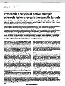
Frequency-Agile Distributed-Sensor System (FADSS) Deployment in the Western United States: VLF Results D. D. Rice, J. V. Eccles, J. J. Sojka, J. W. Raitt, Space Environment Corporation 221 N. Spring Creek Parkway, Suite A, Providence UT 84332-9791 R. D. Hunsucker, R P Consultants, 7917 Gearhart Street Klamath Falls, OR 97601 ABSTRACT A network of inexpensive, frequency-agile, beacon monitors is currently being developed to provide a real-time description of space weather effects on ionospherically-dependent systems. This array of software radios is dynamically programmed to measure GPS variations and received signal strengths from select beacons from VLF through HF along a multitude of propagation paths. The real-time network collects the information and augments it with geophysical data (GOES, various indices.) Processing provides information on the prevailing ionospheric weather conditions, and allows the scheduling of sensor observations to be optimized. We describe the VLF signal strength results of our initial six-station deployment. The initial FADSS frequency selection includes Navy VLF stations in Washington, North Dakota, Hawaii, and Maine. The sensors are deployed in the Western United States: KFO (Klamath Falls, Oregon), BLO (Bear Lake Observatory, Utah), PRV (River Heights, Utah), LGN (Logan, Utah), TUC (Tucson, Arizona), and SEC (at SEC office in Providence, Utah.) Additional beacon monitors are being fabricated for temporary observing campaigns. In this study these measurements are augmented by almost two years of monitoring from Providence, Utah by receivers of the Stanford IHY program. The data show strong seasonal effects on the D-region during solar minimum conditions. In summer, daytime signal levels are quite constant except during Sudden Ionospheric Disturbances (SIDs) related to solar x-ray flares. At night, signal levels are highly variable with gravity wave periods of 1-2 hours dominating. In winter, daytime VLF signal strengths are modulated with periods consistent with planetary waves of several days to more than a week. This modulation also affects signals at low HF frequencies through D-region absorption. The multi-point FADSS measurements are used to deduce the scale lengths of the D-region structures. This information is used to improve ionospheric specification as well as generate knowledge on the scale sizes of these space weather-related ionospheric structures. 1. INTRODUCTION A frequency-agile distributed-sensor system (FADSS) consisting of inexpensive radio beacon monitors is being developed to evaluate propagation conditions from VLF through HF and infer space weather effects. Each monitor is based on a software receiver covering 9 kHz to 30 MHz, equipped with a compact active antenna. A GPS receiver provides accurate time and location information, and may provide additional data about ionospheric disturbances through analysis of reported position variations for a fixed location. A typical beacon monitor is shown in Figure 1. The monitoring system consists of a network distributed across Utah, Oregon, and Arizona (Figure 2) with additional units that can be set up in other locations for observing campaigns. Receivers were deployed between September and November 2007; their coordinates are listed in 1
Table 1. There are also two fixed-frequency VLF receivers operated by Utah State University in the Providence, Utah area that are part of the Stanford International Heliospheric Year (IHY) SID project. Those receivers provided initial VLF observations during the design phase of the present study, and continue to provide supplementary observations. Numerous studies of VLF propagation have been carried out over the years, but most have focused on long paths of several thousand kilometers. Long paths tend to average out smaller-scale ionospheric weather effects, allowing large-scale behavior such as solar flare impacts to be studied. The purpose of this project is to study the smaller-scale effects (e.g., gravity waves, absorption anomalies) and to characterize specific geographical sections of the ionosphere. Thus we emphasize short signal paths, less than about 2000 km.
Figure 1. Typical beacon monitor consisting of a Linux PC with a PCI-based software radio installed. The GPS receiver is sitting on the PC case, and the wideband active antenna is leaning against the PC. The GPS receiver and active antenna are installed outdoors at roof level when the monitor is deployed. TABLE 1. Primary beacon monitoring locations. Receiver
Location
North Latitude East Longitude Altitude, m
BLO
Bear Lake Observatory, UT
41.934
-111.421
1973
KFO
Klamath Falls, Oregon
42.173
-121.850
1320
LGN
Logan, Utah
41.731
-111.807
1460
PRV
River Heights, Utah
41.720
-111.822
1395
SEC
Providence, Utah
41.712
-111.830
1383
TUC
Tucson, Arizona
32.437
-110.982
875
2
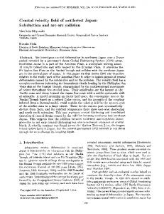
Figure 2. Observational network completed in November 2007 showing northern Utah (left) and the southwestern US (right.) Shaded areas are populated regions. The cluster of systems in the Logan/Providence area is used for development and testing. The primary VLF transmitters monitored for this project are NML (25.2 kHz) in La Moure, North Dakota and NLK (24.8 kHz) in Jim Creek, Washington. These transmitters provide the relatively short paths to the receivers. Longer paths to NAA (24.0 kHz) in Cutler, Maine and NPM (21.4 kHz) in Lualualei, Hawaii are also monitored, since they may help characterize large-scale phenomena. The paths are shown in Figure 3, and distances between the VLF transmitters and receivers are shown in Table 2. Two HF transmitters, WWV and WWVH, are shown in Figure 3 and are also monitored as part of this project, and HF signal absorption is used as another diagnostic of D-region density. In addition, monitoring of NAU (40.8 kHz) in Puerto Rico and WWVB (60 kHz) in Fort Collins is planned for the near future. Besides providing additional signal paths, NAU and WWVB are in the LF range and should exhibit different propagation characteristics than the currently-monitored VLF signals. TABLE 2. Distances between receivers and VLF transmitters in km. Receiver NAA 24.0 kHz NLK 24.8 kHz NML 25.2 kHz BLO 3540 1080 1155 KFO 4335 670 1920 LGN 3580 1070 1190 PRV 3580 1070 1195 SEC 3580 1070 1195 TUC 3980 1980 1885
NPM 21.4 kHz 4900 4085 4860 4860 4860 4795
2. SEASONAL VARIATIONS IN VLF SIGNALS For path lengths of less than 2000 km, diurnal and seasonal variations in VLF signal strength are quite sensitive to the path length. The signal strength for a given path depends on the effective reflection height H’ of the earth-ionosphere waveguide, and analysis of H’ variations with the Long Wave Propagation Capability (LWPC) [Ferguson, 1998] shows that certain combinations of H’ and sharpness β produce signal strength minima and maxima for the path.
3
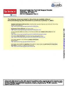
Figure 3. VLF transmitter/receiver paths that are currently monitored. WWV/WWVH HF transmissions are also monitored for this project. The complete 2007 VLF data set of the NML to PRV path obtained from the Stanford IHY SID receiver is shown in Figure 4. The signal strength is shown as a function of UT and day of year. The very distinctive hourglass shape is due to the seasonal variation of daylight hours. The area inside the hourglass shape is nighttime, where maximum signal levels are usually observed. The narrowest section of the hourglass is summer solstice. The bottom of the hourglass is January, and the top is December. The series of regularly-spaced black horizontal stripes between 1200 and approximately 2000 UT represent once-per-week maintenance outages of the NML transmitter. White areas are missing data caused by failures at the receiver site. For the NML-PRV path, LWPC shows a well-defined signal strength minimum associated with H’ ~ 84 km for normal ranges of β. Daytime H’ values are ~72 km, and nighttime values are ~90 km. Thus at dawn and dusk, H’ passes through the minimum signal region, producing the sharp border of the hourglass shape. The dawn crossing (right side) is sharper than the dusk crossing, and is sharpest in summer. This behavior is consistent with the solar zenith angle changing more rapidly during summer dawn than during winter dawn. The dusk crossing is indistinct at times during the winter, suggesting that the β value is large enough at dusk to prevent the significant signal minimum from occurring. Some seasonal effects in Figure 4 have less obvious causes. Daytime signal levels increase abruptly in mid-April and decrease again in October. A gradual shift between winter and summer signal levels is expected due to higher summer sun angles, but the abrupt change suggests that another cause, such as a seasonal change in mesospheric wind patterns. The nighttime signal levels reach much higher levels in the summer, but also have much greater variability, with nighttime signals erratically dropping below daytime levels. The greater summertime variability could be due to H’ being lower in summer than in winter, near the very sensitive range of H’~84 km where the signal strength minimum occurs on the NML-PRV path. For a summer H’ ~87 km, vertical 4
motions due to winds and waves would produce larger signal variations than for a winter H’ of 90 km.
Figure 4. Signal strength observations for 2007 from the Stanford NML receiver in Providence, Utah. Again, the behavior shown in Figure 4 is specific to the NML-PRV path. The seasonal behavior is actually quite similar in the NLK-PRV data, which has a similar path length, but diurnal signal changes in KFO and TUC data are very different due to differing earth-ionosphere waveguide lengths and geometries. For example, the NLK-KFO data has a strong signal 5
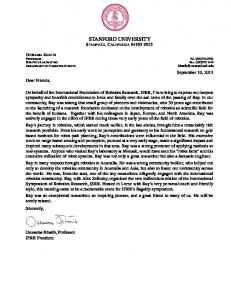
enhancement at dawn and dusk rather than a minimum, while NML-KFO, NML-TUC, and NLKTUC paths have very subtle changes in signal levels at dawn and dusk. 3. WEATHER VARIATIONS IN VLF SIGNALS The year 2007 shown in Figure 4 proved to be a particularly quiet solar minimum year, with few significant solar flares and modest geomagnetic activity. Close inspection of the daytime signal (outside of the hourglass) reveals the few sudden ionospheric disturbances (SIDs) that occurred as short stripes of enhanced signal; for example, two flare SIDs occurred on June 1. Figure 5 shows the signal strength as a function of UT hour at PRV for two transmitters on June 1, 2007, when two solar flares produced classic sudden ionospheric disturbance (SID) signatures. The two transmitters are NML (left) and NLK (right), located in North Dakota and Washington State respectively (Figure 3.) GOES x-ray solar data indicate that the 1500 UT flare was C9 class, and the 2150 UT flare was C8 class. Thomson et al [2005] have studied how the bottomside of the D-region is lowered depending on the class of the x-ray flare, and together with D-region physics models, a good estimate of the ionospheric response is available. For the NMLPRV path, the two SIDs have about the same amplitudes, while the first SID on the NLK-PRV path has a much lower amplitude than the second. The paths have different geometries, with the NLKPRV path being 125 km shorter than the NML-PRV path, but the major difference between the two paths in this case is the solar zenith angle. A solar zenith angle dependence for the D-region bottomside has been found and quantified by McRae and Thomson [2000]. In this case, the first flare occurs earlier in the morning on the NLK-PRV path than on the NML-PRV path, and thus experiences a smaller x-ray enhancement.
Figure 5. Signal strength in Providence Utah for NML (left) and NLK (right) showing sudden ionospheric disturbance (SID) signatures at 1500 and 2200 UT corresponding to solar x-ray flares. Another weather phenomenon visible in Figure 4 is bands of enhanced signal during the winter night (specifically from mid-October to December 2007) that are several days apart (compare with the weekly transmitter downtime stripes.) The timing of these enhancements is consistent with planetary wave periods, and may result from NO transport from higher latitudes associated with the waves [Kawahira, 1985]. Some of these night VLF enhancements correlate with daytime HF signal absorption (Figure 6), showing that the changes in the D-region persist through the day, and suggesting a connection to the winter absorption anomaly that has been observed at HF for decades. The VLF path is well northwest of the HF path, but on several occasions (25-27 December 2007, 31December-2 January 2008, 26 January-6 February 2008) nighttime VLF increases corresponded to daytime HF absorption. 6
A key question for FADSS is the geographic distribution and extent of ionospheric weather variations. For solar flare effects, the extent is assumed to be the entire dayside hemisphere, but for planetary wave-driven NO enhancements, studies of absorption suggest that scale sizes are less than 500 km [Schwentek, 1974]. Smaller scale variations on the order of tens to hundreds of kilometers are produced by atmospheric gravity waves; see Taylor et al. [2007] for examples of optical mesospheric gravity wave observations at BLO. It is hoped that analysis of the various paths in the FADSS, and the overlaps in the path data, will allow for a more detailed ionospheric specification that will provide new information about the scale sizes and distributions of D-region irregularities. Clearly, more sensors are needed, and short-term mobile campaigns are planned to collect data from various locations across the Western United States during the next year.
Klamath Falls Signal -5 -10
Signal, dB
-15 -20 10 MHz Day NLK Night
-25 -30 -35 -40 1201
1208
1215
1222
1229
0105
0112
0119
0126
0202
0209
0216
0223
0301
Month/Day, 2007-2008
Figure 6. Comparison of average night VLF and day HF signal observed at KFO. Low HF signal levels reflect increased D region absorption. 4. CORRELATION SCALES OF VLF OBSERVATION The current FADSS deployment has two scales, shown in Figure 2: the cluster shown in the left panel of the figure and the wide-area network shown in the right panel. Comparing the signals from these receivers shows how the signals correlate over short ranges, and limiting the comparison to night (about 0030-1330 UT for early January in Utah) eliminates differences in solar zenith angle along the paths. Nighttime signals from NML received by the cluster of receivers in the Logan, Utah area are shown in Figure 7. Data points are at three-minute intervals, and correlated variations are seen on various time scales, ranging from about 15 minutes through several hours. The BLO receiver shows the least correlation, and it is the farthest from the cluster (42 km from SEC.) The other receivers are within about 5 km of each other. 7
NML, 5 Jan 2008 -10
-15
-20
BLO LGN
-25
PRV SEC
-30
-35
-40 0
3
6
9
12
15
UT Hour
Figure 7. Signal correlations between receivers in a 50 km-wide area. The correlated variations in Figure 7 have periods typical of atmospheric gravity waves and long-period inertial or tidal waves after 0600 UT. The 42 km distance between BLO and the other monitors is comparable to short-scale gravity wavelengths, and is about three signal wavelengths, so small differences between the received signal at BLO and the other monitors are reasonable. Differences between the LGN/PRV/SEC monitors are most likely due to local interference, variations in antenna characteristics, and system noise. Signals from NML to the three remote receivers at BLO (Utah), KFO (Oregon), and TUC (Arizona) are shown in Figure 8. While all three signals show wave-like variations, there is no obvious correlation between them. The paths are widely separated (see Figure 3) so there are differences in dawn and dusk times and potentially different weather conditions along the paths due to wind and wave effects. We would not generally expect obvious correlations between distant receivers. Even assuming a wide-area disturbance that affects the signal paths in the same way (such as a solar flare), the resulting signal fluctuations will have different signatures at different locations due to differing patterns of constructive and destructive interference between modes along the waveguide. Figure 9 illustrates this situation: an M2-class solar flare at 1900 produces a simple increase in signal on the NLK-PRV path, but produces an initial sharp decrease in signal on the NLK-KFO path followed by an increase. Ideally, these differences will be accounted for through the LWPC modeling analysis. Atmospheric waves will complicate the analysis, however, since wavelengths and directions of the waves are unknown, so the amplitude variation due to the atmospheric waves across the various signal paths is also unknown. It is hoped that waves with large amplitudes and wavelengths may be identified using multiple overlapping signal paths, but the optimal arrangement and spacing of signal paths remains to be determined. 8
NML, 5 Jan 2008 -10
-15
-20
BLO -25
KFO TUC
-30
-35
-40 0
3
6
9
12
15
UT Hour
Figure 8. Signal correlations across the Western United States.
Figure 9. SID from x-ray flare at 1900 UT observed in Klamath Falls (left) and Providence (right.) Dark vertical lines indicate local dawn and dusk. 5. CONCLUSIONS Long-term observations of fixed VLF transmitter-receiver signal paths can provide valuable information about weather in the D-region. Analysis of the signal data requires a suitable waveguide propagation model such as LWPC, and an ionospheric model that provides information about the expected quiet-time diurnal and seasonal variations. Once the baseline has been established for signals under quiet conditions, large perturbations in the signal may be mapped to ionospheric weather. This study has collected examples of various signal perturbations and is currently developing the analysis tools that will yield the ionospheric weather information.
9
The next step is to use the overlapping signal paths of the sensor network to estimate the location and extent of the inferred weather phenomena. A variety of signal paths will be examined with field campaigns during the next year. Data gathered so far have demonstrated connections between VLF propagation and HF absorption, and are being used to improve the AbbyNormal D-region model. Close examination of solar x-ray flare responses in these data sets have also suggested that assumptions about flare spectrum and D-region response will need to be revisited. In all, FADSS observations promise to make significant contributions to the understanding of D-region physics. Acknowledgement: This research was supported by SBIR II Contract FA8718-07-C-0016 from AFRL at Hanscom AFB to the Space Environment Corporation. The assistance and support of Dr. Robert D. Hunsucker and Dr. John W. Raitt was essential to the success of this campaign. The VLF SID Space Weather Monitor is an instrument developed through a project sponsored by Stanford University, the National Science Foundation, NASA, and is part of the United Nations’ International Heliospherical Year, 2007. See http://sid.stanford.edu for project information and data distribution. References Ferguson, K., Computer Programs for Assessment of Long-Wavelength Radio Communications, Version 2.0, Technical Document 3030, May 1998, Space and Naval Warfare Systems Center, San Diego, CA 92152-5001, 1998. Kawahira, K., The D region winter anomaly at high and middle latitudes induced by planetary waves, Radio Sci., 20, 795-802, 1985. McRae, W. M. and N. R.Thomson, VLF phase and amplitude: daytime ionospheric parameters, J. Atmos. Solar-Terr. Phys., 62, 609-618, 2000. Schwentek, H., Some results obtained from the European cooperation concerning studies of the winter anomaly in ionospheric absorption, COSPAR Proceedings of the Methods of Measurements and Results of Lower Ionosphere Structures Symposium held in Constance, F.R.G, edited by K. Rawer, 281-286, 1974. Taylor, M. J., W. R. Pendleton Jr., P-D. Pautet, Y. Zhao, C. Olsen, H. K. S. Babu, A. F. Medeiros, and H. Takahashi, Recent progress in mesospheric gravity wave studies using nightglow imaging system, Rev. Bras. Geof., 25(2), 49-58, doi: 10.1590/S0102-261X2007000600007, 2007. Thomson, N. R., C. J. Rodger, and M. A. Clilverd, Large solar flares and their ionospheric Dregion enhancements, J. Geophys. Res., 110, A06306, doi:10.1029/2005JA011008, 2005.
10