Jul 19, 2013 - Krishnaswami et al. employ a more expressive notion of recursion, which entails unique fixed points [20â22]. This means that their type systems ...
Fair Reactive Programming Andrew Cave
Francisco Ferreira
Prakash Panangaden
Brigitte Pientka
McGill University {acave1,fferre8,prakash,bpientka}@cs.mcgill.ca
Abstract
erties) for least and greatest fixed points, in the spirit of the modal µ-calculus [19]. The “always”, “eventually” and “until” modalities of LTL arise simply as special cases. We do this while still remaining relatively conservative over LTL. Moreover, we demonstrate that distinguishing between and interleaving of least and greatest fixed points is key to statically guarantee liveness properties, i.e. something will eventually happen, by type checking. To illustrate the power and elegance of this idea, we describe the type of a fair scheduler – any program of this type is guaranteed to be fair, in the sense that each participant is guaranteed that his requests will eventually be served. Notably, this example requires the expressive power of interleaving least fixed points and greatest fixed points, a construction due to Park [28], and which is unique to our system. Our approach of distinguishing between least and greatest fixed points and allowing for iteration and coiteration is in stark contrast to prior work in this area: Jeffrey’s work [14, 15] for example only supports less expressive combinators instead of the primitive (co)recursion our system affords, and only particular instances of our recursive types. Krishnaswami et al. employ a more expressive notion of recursion, which entails unique fixed points [20–22]. This means that their type systems are actually less expressive, in the sense that they cannot guarantee liveness properties about their programs. Our technical contributions are as follows:
Functional Reactive Programming (FRP) models reactive systems with events and signals, which have previously been observed to correspond to the “eventually” and “always” modalities of linear temporal logic (LTL). In this paper, we define a constructive variant of LTL with least fixed point and greatest fixed point operators in the spirit of the modal mu-calculus, and give it a proofs-asprograms interpretation in the realm of reactive programs. Previous work emphasized the propositions-as-types part of the correspondence between LTL and FRP; here we emphasize the proofsas-programs part by employing structural proof theory. We show that this type system is expressive enough to enforce liveness properties such as the fairness of schedulers and the eventual delivery of results. We illustrate programming in this language using (co)iteration operators. We prove type preservation of our operational semantics, which guarantees that our programs are causal. We give also a proof of strong normalization which provides justification that the language is productive and that our programs satisfy liveness properties derived from their types. Categories and Subject Descriptors D.3.2 [Programming Languages]: Language Classifications – Applicative (functional) languages
1.
Introduction • A type system which, in addition to enforcing causality (as in
Reactive programming seeks to model systems which react and respond to input such as games, print and web servers, or user interfaces. Functional reactive programming (FRP) was introduced by Elliott and Hudak [9] to raise the level of abstraction for writing reactive programs, particularly emphasizing higher-order functions. Today FRP has several implementations [6–8, 27]. Many allow one to write unimplementable non-causal functions, where the present output depends on future input, and space leaks are all too common. Recently there has been a lot of interest in type-theoretic foundations for (functional) reactive programming [13, 16, 20–22] with the intention of overcoming these shortcomings. In particular, Jeffrey [13] and Jeltsch [16] have recently observed that Pnueli’s linear temporal logic (LTL) [29] can act as a type system for FRP. In this paper, we present a novel logical foundation for discrete time FRP with (co)iteration operators which exploits the full expressiveness afforded by the proof theory (i.e. the universal prop-
previous systems [13, 21]), also enables one to enforce liveness properties; fairness being a particularly intruiging example. Moreover, our type system forms a sound proof system for LTL. While previous work [13] emphasized the propositionsas-types component of the correspondence between LTL and FRP, the present work additionally emphasizes the proof-asprograms part of the correspondence through the lens of structural proof theory. Our type system bears many similarities to Krishnaswami’s recent work [20]. The crucial difference lies in the treatment of recursive types and recursion. Our work distinguishes between least and greatest fixed points, while Krishnaswami’s work collapses them. • A novel operational semantics which provides a reactive in-
tepretation of our programs. One can evaluate the result of a program for the first n time steps, and in the next time step, resume evaluation for the (n + 1)st result. It allows one to evaluate programs one time step at a time. Moreover, we prove type preservation of our language. As a consequence, our language is causal: future inputs do not affect present results. • A strong normalization proof using Tait’s method of saturated
sets which justifies that our programs are productive total functions. It also demonstrates that our programs satisfy liveness properties derived from their types. Notably, our proof tackles the full generality of interleaving fixed points, and offers a novel treatment of monotonicity.
[Copyright notice will appear here once ’preprint’ option is removed.]
1
2013/7/19
2.2
The paper is organized as follows: To illustrate the main idea, limitations and power of our foundation, we give several examples in Sec. 2. In particular, we elaborate the implementation of two fair schedulers where our foundation statically guarantees that each request will eventually be answered. We then introduce the syntax (Sec. 3) of our language which features (co)iteration operators and explicit delay operators together with typing rules (Sec. 4). In Sec. 5 we describe the operational semantics and prove type preservation. In Sec. 6, we outline the proof of strong normalization. In Sec. 7, we discuss consequences of strong normalization and type preservation, namely causality, liveness, and productivity. We conclude with related work.
2.
A key feature of our foundation is the distinction between least fixed points and greatest fixed points. In other words, the distinction between data and codata. This allows us to make a distinction between events that may eventually occur and events that must eventually occur. This is a feature not present in the line of work by Krishnaswami and his collaborators, Benton and Hoffman [20– 22] – they have unique fixed points corresponding most closely to our greatest fixed points. To illustrate the benefits of having both, least and greatest fixed points, we present here the definition of LTL’s ♦ operator (read: “eventually”) as a data type, corresponding to a type of events in reactive programming:
Examples
data ♦ A = Now of A | Later of ♦ A
To illustrate the power of our language, we first present several motivating examples using an informal ML or Haskell-like syntax. For better readability we use general recursion in our examples, although our foundation only provides (co)iteration operators. However, all the examples can be translated into our foundation straightforwardly and we subsequently illustrate the elaboration in Sec 3. On the type level, we employ a type constructor corresponding to the “next” modality of LTL to describe data available in the next time step. On the term level, we use the corresponding introduction form • and elimination form let • x = e in e’ where x is bound to the value of the expression e in the next time step. 2.1
The “eventually” modality
The function evapp below receives an event of type A and a time-varying stream of functions A → B. It produces an event of type B. Operationally, evapp waits for the A to arrive, applies the function available at that time, and fires the resulting B event immediately: evapp : ♦ A evapp ea fs | Now x | Later ea’
The “always” modality
→ �(A → B) → ♦ B = case ea of ⇒ Now ((hd fs) x) ⇒ let • ea’’ = ea’ • fs’ = tl fs in Later (• (evapp ea’’ fs’))
This is not the only choice of implementation for this type. Such functions could opt to produce a B event before the A arrives, or even long after (if B is something concrete such as bool). However, all functions with this type (in our system) have the property that given that an A is eventually provided, it must eventually produce a B, although perhaps not at the same time. This is our first example of a liveness property guaranteed by a type. This is in contrast to the “weak eventually” modality present in other work, which does not guarantee the production of an event. It is interesting to note that this program (and all the other programs we write) can rightly be considered proofs of their corresponding statements in LTL.
Our first example app produces a stream of elements of type B, given a stream fs of functions of type A → B and a stream xs of elements of type A by applying the nth function in fs to the nth value in xs. Such streams are thought of as values which vary in time. Here we use the � type of LTL to describe temporal streams, where the nth value is available at the nth time step. � A can be defined in terms of the modality as follows using a standard definition as a greatest fixed point (a coinductive datatype). codata � A = _::_ of A × � A
� A has one constructor :: which is declared as an infix operator and takes an A now and recursively a � A in the next time step. The functions hd and tl can then be defined, the only caveat being that the type of tl expresses that the result is only available in the next time step:
2.3
Abstract server
Here we illustrate an abstract example of a server whose type guarantees responses to requests. This example is inspired by a corresponding example in Jeffrey’s [15] recent work. We wish to write a server which responds to two kinds of requests: Get and Put with possible responses OK and Error. We represent these:
hd : � A → A tl : � A → � A
data data
Finally, we can implement the app function as follows:
Req = Get | Put Resp = OK | Error
At each time step, a server specifies how to behave in the future if it did not receive a request, and furthermore, if it receives a request, it specifies how to respond and also how to behave in the future. This is the informal explanation for the following server type, expressed as codata (here, we use coinductive record syntax):
app : � (A → B) → � A → � B app fs xs = let • fs’ = tl fs • xs’ = tl xs in ((hd fs) (hd xs)) :: (• (app fs’ xs’))
codata
We use the elimination form, let • to bind the variables fs’ and xs’ to values of the remaining streams in the next time step. Our typing rules will guarantee that fs’ and xs’ are only usable underneath a •, which we will explain further in the following examples. Such a program is interpreted reactively as a process which, at each time step, receives a function A → B and a value A and produces a value B. More generally, given n functions A → B and n values A, it can compute n values B.
Server = {noreq : Server, some : Req → Resp × Server}
Now we can write the server program which responds to Get with OK and Put with Error: server : Server server = { noreq = • server, some = λr. if isGet r then (OK, • server) else (Error, • server)}
2
2013/7/19
Our language does not have Nakano’s guarded recursion [12] fix : ( A → A) → A because it creates for us undesirable inhabitants of inductive types (inductive types collapse into coinductive types). For example, the following would be an undesirable inhabitant of ♦A in which the A is never delivered:
Above, we say that if no request is made, we behave the same in the next time step. If some request is made, we check if it is a Get request and respond appropriately. In either case, in the next time step we continue to behave the same way. More generally, we could opt to behave differently in the next time step by e.g. passing along a counter or some memory of previous requests. It is clear that this type guarantees that every request must immediately result in a response, which Jeffrey calls a liveness guarantee. In our setting, we reserve the term liveness guarantee for something which has the traditional flavor of “eventually something good happens”. That is, they are properties which cannot be falsified after any finite amount of time, because the event may still happen. The present property of immediately providing a response does not have this flavor: it can be falsified by a single request which does not immediately receive a response. In our setting, liveness properties arise strictly from uses of inductive types (i.e. data, or µ types) combined with the temporal modality, which requires something to happen arbitrarily (but finitely!) far into the future. 2.4
never : ♦ A never = fix (λx. Later x)
−− disallowed
Finally, the following program which attempts to build a constant stream cannot be elaborated into the formal language. While it is guarded, we must remove all local variables from scope in the bodies of recursive definitions, so the occurrence of x is out of scope. repeat : A → � A repeat x = xs where xs = x :: •xs
−− x out of scope !
This is intentional – the above type is not uniformly a theorem of LTL, so one should not expect it to be inhabited. As Krishnaswami et al. [22] illustrate, this is precisely the kind of program which leads to space leaks.
Causality-violating (and other bad) programs
We wish to disallow programs such as the following, which has the effect of pulling data from the future into the present; it violates a causal interpretation of such programs. Moreover, its type is certainly not a theorem of LTL for arbitrary A!
2.5
Fair scheduling
Here we define a type expressing the fair interleavings of two streams, and provide examples of fair schedulers employing this type – this is the central example illustrating the unique power of the presented system. This is enabled by our system’s ability to properly distinguish between and interleave least and greatest fixed points (i.e. data and codata). Other systems in the same vein typically collapse least fixed points into greatest fixed points or simply lack the expressiveness of recursive types. First we require the standard “until” modality of LTL, written A U B. This is a sequence of As, terminated with a B. In the setting of reactive programming, Jeltsch [17] calls programs of this type processes – they behave as time-varying signals which eventually terminate with a value.
predictor : A → A predictor x = let • x’ = x in x’ −− does not typecheck Our typing rules disallow this program roughly by restricting variables bound under a • to only be usable under a •, in much the same way as Krishnaswami [20]. Similarly, the type (A + B) expresses that either an A or a B is available in the next time step, but it is not known yet which one it will be. Hence we disallow programs such as the following by disallowing case analysis on something only available in the future:
data
predictor : (A + B) → A + B predictor x = let • x’ = x in case x’ of −− does not typecheck | inl a ⇒ inl (• a) | inr a ⇒ inr (• b)
A U B = Same of A × ( (A U B)) | Switch of B
Notably, since this is an inductive type, the B must eventually occur. The coinductive variant is “weak until”; the B might never happen, in which case the As continue forever. We remark that without temporal modalities, A U B is isomorphic to (List A) × B, but because of the , it matters when the B happens. We define also a slightly stronger version of “until” which requires at least one A, which we write A Uˆ B.
Such a program would tell us now whether we will receive an A or a B in the future. Again this violates causality. Due to this interpretation, there is no uniform inhabitant of this type, despite being a theorem of classical LTL. Similarly, ⊥ → ⊥ is uninhabited in our system; one cannot get out of doing work today by citing the end of the world tomorrow. Although it would be harmless from the perspective of causality, we disallow also the following:
type
A Uˆ B = A × (A U B)
We characterize the type of fair interleavings of a stream of A s and Bs as some number of As until some number of Bs (at least one), until an A, and the process restarts. This is fair in the sense that it guarantees infinitely many As and infinitely many Bs. As a coinductive type:
import : A → A import x = • x −− does not typecheck This is disallowed on the grounds that it is not uniformly a theorem of LTL. Krishnaswami and Benton allow it in [21], but disallow it later in [22] to manage space usage. Syntactically, this is accomplished by removing from scope all variables not bound under a • when moving under a •. However, some concrete instances of this type are inhabited, for example the following program which brings natural numbers into the future:
codata
Fair A B = In of (A U (B Uˆ (A × (Fair A B))))
This type corresponds to the B¨uchi automaton in Figure 1. With this type, we can write the type of a fair scheduler which takes a stream of As and a stream of Bs and selects from them fairly. Here is the simplest fair scheduler which simply alternates selecting an A and B:
import : Nat → Nat import Zero = • Zero import (Succ n) = let • n’ = import n in •(Succ n’)
sched : � A → � B → Fair A B sched as bs =
3
2013/7/19
a
b
b
qa
mutual
cnt : TNat → TNat → � A → � B → (A U (B Uˆ (A × (Fair A B)))) cnt n m as bs = let • m’ = import m • as’ = tl as • bs’ = tl bs
qb
� start
in case
a
n of | Zero ⇒ Switch (hd bs, • (Switch (hd as’, let • m’’ = import m’ • as’’ = tl as’ • bs’’ = tl bs’
q0
Figure 1. Scheduler automaton.
in
let • as’ = tl as
• (sch2’ (Succ (import m’’)) as’’ bs’’))) | Succ p ⇒ let • n’ = p in Same (hd as, (• (cnt n’ m’ as’ bs’)))
• bs’ = tl bs in
In (Switch (hd bs, • (Switch (hd as’, let • as’’ = tl as’ • bs’’ = tl bs’ in • (sched as’’ bs’’)))))
and
sch2’ : TNat → � A → � B → Fair A B sch2’ n as bs = In (cnt n n as bs) −− Main function sch2 : � A → � B → Fair A B sch2 as bs = sch2’ Zero as bs
The reader may notice that this scheduler drops the As at odd position and the Bs at even position. This could be overcome if one has import for the corresponding stream types, but at the cost of a space leak. as :
a
a
a
a
a
a
a
a
a
a
a
a
a
a
bs :
b
b
b
b
b
b
b
b
b
b
b
b
b
b
Figure 2. Fair scheduler
3.
The formal syntax for our language (Figure 3) includes conventional types such as product types, sum types and function types. Additionally the system has the A modality for values which will have the type A in the next step and least and greatest fixed points, µ and ν types. Our convention is to write the letters A, B, C for closed types, and F, G for types which may contain free type variables.
However, this “dropping” behaviour could be viewed positively: in a reactive setting, the source of the A requests could have the option to re-send the same request or even modify the previous request after observing that the scheduler decided to serve a B request instead. Next we illustrate a more elaborate implementation of a fair scheduler which serves successively more As each time before serving a B. Again the type requires us to eventually serve a B. as :
a
a
a
a
a
a
a
a
a
a
a
a
a
a
bs :
b
b
b
b
b
b
b
b
b
b
b
b
b
b
Types A, B, F, G
::=
1|F ×G|F +G|A→F |
F | µX.F | νX.F | X
Terms M, N ::= x | () | (M, N ) | fst M | snd M | | inl M | inr M | case M of inl x 7→ N | inr y 7→ N 0 | λx.M | M N | •M | let • x = M in N | inj M | iterX.F (x.M ) N | out M | coitX.F (x.M ) N | map (∆.F ) η M
We will need a special notion of “timed natural numbers” to implement the countdown. In the Succ case, the predecessor is only available in the next time step: data
Syntax
TNat = Zero | Succ ( TNat)
Contexts Θ, Γ Kind Contexts ∆ Type substitutions ρ Morphisms η
We can write a function which imports TNats: import : TNat → TNat
::= ::= ::= ::=
· | Γ, x : A · | ∆, X : ∗ · | ρ, F/X · | η, (x.M )/X
Figure 3. LTL Syntax
The scheduler is implemented in Figure 2. It involves two mutually recursive functions: cnt is structurally decreasing on a TNat, counting down how many As to produce, while the recursive call to sch2’ is guarded by the necessary Switchs to guarantee productivity, and increments the number of As served the next time. sch2 kicks off the process starting with zero As. To understand why type TNat is necessary, we note cnt is structurally decreasing on its first argument. This requires the immediate subterm n’ to be available in the next step, not the current. The important remark here is that these schedulers can be seen to be fair simply by virtue of typechecking and termination/productivity checking. More precisely, this is seen by elaborating the program to use the (co)iteration operators available in the formal language, which we illustrate in the next section.
Our term language is mostly standard and we only discuss the terms related to modality and the fixed points, µ and ν. •M describes a term M which is available in the next time step. let • x = M in N allows us to use the value of M which is available in the next time step in the body N . Our typing rules will guarantee that the variable only occurs under a •. Our language also includes iteration operator iterX.F (x.M ) N and coiteration operator coitX.F (x.M ) N . Intuitively, the first argument x.M corresponds to the inductive invariant while N specifies how many times to unroll the fixed point. The introduction form for µ types is inj M , rolling up a term M . The elimination form for ν types is out M , unrolling M .
4
2013/7/19
We note that the X.F annotations on iter and coit play a key role during runtime, since the operational semantics of map are defined using the structure of F (see Sec. 5). We do not annotate λ abstractions with their type because we are primarily interested in the operational behaviour of our language, and not e.g. unique typing. The term map (∆.F ) η N witnesses that F is a functor, and is explained in more detail in the next sections. Our type language with least and greatest fixed points is expressive enough that we can define the always and eventual modality e.g.:
Well-formedness of types: ∆ ` F : ∗ ∆`1:∗
(X : ∗) ∈ ∆ ∆`F :∗ ∆ ` F : ∗ ∆ ` X : ∗
Figure 4. Well-formed types
Typing Rules for →, ×, +, 1 Θ; Γ, x : A ` M : B Θ; Γ ` λx.M : A → B x:A ∈ Γ Θ; Γ ` x : A
Θ; Γ ` M : A Θ; Γ ` N : B Θ; Γ ` (M, N ) : A × B
Θ; Γ ` M : A × B Θ; Γ ` snd M : B
Θ; Γ ` M : A Θ; Γ ` inl M : A + B
Θ; Γ ` N : B Θ; Γ ` inr N : A + B
Θ; Γ ` M : A + B Θ; Γ, x : A ` N1 : C Θ; Γ, y : B ` N2 : C Θ; Γ ` case M of inl x 7→ N1 | inr y 7→ N2 : C Rules for modality and least and greatest fixed points Θ; Γ ` M : A Θ, x : A; Γ ` N : C Θ; Γ ` let • x = M in N : C
·; Θ ` M : A Θ; Γ ` •M : A
Θ; Γ ` M : [µX.F/X]F ·; x : [C/X]F ` M : C Θ; Γ ` N : µX.F Θ; Γ `inj M : µX.F Θ; Γ `iterX.F (x.M ) N: C ·; x : C ` M : [C/X]F
Θ; Γ ` N : C
Θ; Γ ` M : νX.F Θ; Γ `out M : [νX.F/X]F
Θ; Γ `coitX.F (x.M ) N: νX.F ∆ ` F : ∗ Θ; Γ ` M : [ρ1 ]F
ρ1 ` η : ρ2
Θ; Γ ` map (∆.F ) η M : [ρ2 ]F Typing Rules for morphisms: ρ1 ` η : ρ2 ρ1 ` η : ρ2 ·; x : A ` M : B ρ1 , A/X ` η, (x.M )/X : ρ2 , B/X
νX. X × (Req → Resp × X) µX.(B + A × X) A × (A U B) νX.(A U (B Uˆ (A × X)))
·`· : ·
Figure 5. Typing Rules employ a strict positivity restriction, in contrast to Krishnaswami’s guardedness condition [20]. We give a type assignment system for our language in Fig. 5 where we distinguish between the context Θ which provides types for variables which will become available in the next time step (i.e. when going under a •) and the context Γ which provides types for the variables available at the current time. The main typing judgment, Θ; Γ ` M : A asserts that M has type A given the context Θ and Γ. In general, our type system is similar to that of Krishnaswami and collaborators. While in their work, the validity of assumptions at a given time step is indicated either by annotating types with a time [21] or by using different judgments (i.e. now, later, stable) [20], we separate assumptions which are valid currently from the assumptions which are valid in the next time step via two different contexts. We suggest that keeping assumptions at most one step into the future models the practice of reactive programming better than
Finally, to illustrate the relationship between our formal language which features (co)iteration operators and the example programs which were written using general recusion, we show here the program app in our foundation. Here we need to use the pair of f s and xs as the coinduction invariant: app : �(A → B) → �A → �B app f s xs ≡ coitX.B× X (x. let • f s0 = tl (fst x) in let • xs0 = tl (snd x) in ( (hd (fst x)) (hd (snd x)) , •(f s0 , xs0 ) ) ) (f s, xs)
4.
Θ; Γ ` M : A → B Θ; Γ ` N : A Θ; Γ ` M N : B
Θ; Γ ` () : 1
Θ; Γ ` M : A × B Θ; Γ ` fst M : A
inf A ≡ νX.µY.(A× X + Y ) In this definition, at each step we have the choice of making progress by providing an A or postponing until later. The least fixed point implies that one can only postpone a finite number of times. The two definitions are logically equivalent, but have different constructive content – they are not isomorphic as types. Intuitively, �♦A provides, at each time step, a handle on an A to be delivered at some point in the future. It can potentially deliver several values of type A in the same time step. On the other hand, inf A can provide at most one value of type A at each time step. This demonstrates that the inclusion of general µ and ν operators in the language (in lieu of a handful of modalities) offers more finegrained distinctions constructively than it does classically. We show here also the encoding of Server, A U B, A Uˆ B and Fair A B which we used in the examples in Sec. 2.
≡ ≡ ≡ ≡
∆`F :∗ ∆`G:∗ ∆`F +G:∗
· ` A : ∗ ∆ ` F : ∗ ∆, X : ∗ ` F : ∗ ∆, X : ∗ ` F : ∗ ∆`A→F :∗ ∆ ` µX.F : ∗ ∆ ` νX.F : ∗
�A ≡ νX.A × X ♦A ≡ µX.A + X The definition of �A expresses that when we unfold a �A, we obtain a value of type A (the head of the stream) and another stream in the next time step. The definition of ♦A expresses that in each time step, we either have a value of type A now or a postponed promise for a value of type A. The use of the least fixed point operator guarantees that the value is only postponed a finite number of times. Using a greatest fixed point would permit always postponing and never providing a value of type A. We can also express the fact that a value of type A occurs infinitely often by using both great and least fixed points. Traditionally one expresses this by combining the always and eventually modalities, i.e. �♦A. However, there is another way to express this, namely:
Server AU B A Uˆ B Fair A B
∆`F :∗ ∆`G:∗ ∆`F ×G:∗
Type System
We define well-formed types in Fig. 4. In particular, we note that free type variables cannot occur to the left of a →. That is to say, we
5
2013/7/19
a general time-indexed type system. Much more importantly, our foundation differs in the treatment of recursive types and recursion. Most rules are standard. When traversing λx.M , the variable is added to the context Γ describing the fact that x is available in the current time step. Similarly, variables in each of the branches of the case-expression, are added to Γ. The interesting rules are the ones for modality and fixed points µ and ν. In the rule I , the introduction rule for with corresponding constructor •, provides a term to be evaluated in the next time step. It is then permitted to use the variables promised in the next time step, so the assumptions in Θ move to the “available” position, while the assumptions in Γ are no longer available. In fact, the variables in Θ remain inaccessible until going under a • – this is how causality is enforced. Our motivation for forgetting about current assumptions Γ and not allowing them to persist is that we wish to obtain a type system which is sound for LTL. Allowing Γ to persist would make the unsound A → A easily derivable. In the work of Krishnaswami et. al [22], forgetting about current assumptions plays a key role in managing space usage. The corresponding elimination form let • x = M in N simply adds x:A, the type of values promised by M , to the context Θ and we continue to check the body N allowing it to refer to x under a •. The elimination form for µ is an iteration operator iter. Examining an instantiation of this rule for Nat ≡ µX.1 + X may help to clarify this rule:
F (µF )
F (iterf )
f
inj iter f
µF
coitf
F (C)
C
C
νF
f F (C)
out
F (coitf )
F (νF )
We remark that the primitive recursion operator below can be derived from our (co)iteration operators in the standard way, so we do not lose expressiveness by only providing (co)iteration. One can similarly derive a primitive corecursion operator. ·; x : [C × µX.F/X]F ` M : C Θ; Γ ` N : µX.F Θ; Γ ` recX.F (x.M ) N : C The term map (∆.F ) η M witnesses that F is a functor. It has the effect of applying the transformations specified by η at the positions in M specified by F . It is a generic program defined on the structure of F . While this term is definable at the meta-level using the other terms in the language, we opt to include it in our syntax, because doing so significantly simplifies the operational semantics and proof of normalization. In this term, ∆ binds the free variables of F . It is illustrative to consider the case where F (Y ) = list Y = µX.1 + Y × X. If y : A ` M : B and N : list A, then map (Y. list Y ) ((y. M )/Y ) N : list B. In this case, map implements the standard notion of map on lists! We define two notions of substitution: substitution for a “current” variable, written [N/x]M , and substitution for a “next” variable, written [N/x]• M . The key case in their definition is the case for •M . For current substitution [N/x](•M ), in well-scoped terms, x cannot occur in M , so we define:
· ; x : 1 + C ` M : C Θ; Γ ` N : µX.1 + X Θ; Γ `iterX.1+X (x.M ) N : C The term M contains the base case and the step case (M will typically be a case analysis on x), while N specifies how many times to iterate the step case of M starting at the base case of M . For example, we illustrate here the doubling function on natural numbers written using this iteration operator. We write 0 for the term inj (inl ()) and suc m for the term inj (inr m).
[N/x](•M ) = •M For next substitution [N/x]• (•M ), in the body of M , x becomes a current variable, so we can defer to current substitution, defining:
= iterX.1+X (x.case x of inl y 7→ 0 | inr w 7→ suc(suc w)) double = λx:Nat.db x
[N/x]• (•M ) = •([N/x]M ) These definitions are motivated by the desire to obtain tight bounds on how substitution interacts with the operational semantics without having to keep typing information to know that terms are well-scoped. These substitutions satisfy the following typing lemmas.
db
We note that dropping Θ and Γ in the first premise is essential. Intuitively, the bodies of recursive definitions need to be used at arbitrary times, while Γ and Θ are only available for the current and next time steps, respectively. This is easiest to see for the coit rule, where keeping Γ allows a straightforward derivation of A → �A (repeat), which is unsound for LTL and easily produces space leaks. Similarly, keeping Γ in the iter rule allows one to derive the unsound A → ♦B → A U B which says that if A holds now, and B eventually holds, then A in fact holds until B holds.
Lemma 1. Substitution Typing 1. If Θ; Γ, x:A ` M : B and Θ; Γ ` N : A then Θ; Γ ` [N/x]M : B 2. If Θ, x:A; Γ ` M : B and ·; Θ ` N : A then Θ; Γ ` [N/x]• M : B
5.
Operational Semantics
Next, we define a small-step operational semantics for our language using evaluation contexts. Since we allow full reductions, a redex can be under a binder and in particular may occur under a modality. We define evaluation contexts in Fig. 6. We index an evaluation context Ek by a depth k which indicates how many modalities we traverse. Intuitively, the depth k tells us how far we have stepped in time - or to put it differently, at our current time, we know that we have at most taken k time steps and therefore terms under k modalities are available to us now. Single step reduction is defined on evaluation contexts at a time α < ω + 1 (i.e. either α ∈ N or α = ω) and states that we can step Ek [M ] to Ek [N ] where M is a redex occurring at depth k where
unsound : A → ♦B → A U B unsound ≡ λa. λeb. iterX.B+ X (y. case y of |inl b 7→ inj (inl b) |inr u 7→ inj (inr (a, u)) – a out of scope! ) eb The typing rules for µ and ν come directly from the universal properties of initial algebras and terminal coalgebras. The reader may find it clarifying to compare these rules to the universal properties, depicted here:
6
2013/7/19
with these. We sidestep the issue by disallowing reductions inside these bodies. To illustrate the operational semantics and the use of map, we consider an example of a simple recursive program: doubling a natural number.
Ek+1 ::= •Ek Ek ::= Ek N | M Ek | fst Ek | snd Ek | (Ek , M ) | (M, Ek ) | λx.Ek | case Ek of inl x 7→ N | inr y 7→ N 0 | inl Ek | case M of inl x 7→ Ek | inr y 7→ N | inr Ek | case M of inl x 7→ N | inr y 7→ Ek | let • x = Ek in N | let • x = M in Ek | inj Ek | iterX.F (x.M ) Ek | coitX.F (x.M ) Ek | out Ek | map (∆.F ) η Ek E0 ::= []
Example We revisit here the program double which multiplies a given natural number by two given in the previous section. Recall the following abbreviations for natural numbers: 0 =inj (inl ()), suc w =inj (inr w), 1 = suc 0, etc. Let us first compute double 0.
Figure 6. Evaluation contexts
double 0 −→ db (inj (inl ()) −→ case M0 of inl y 7→ 0 | inr w 7→ suc (suc w)
(λx.M ) N −→ [N/x]M fst (M, N ) −→ M snd (M, N ) −→ N case (inl M ) of inl x 7→ N1 | inr y 7→ N2 −→ [M/x]N1 case (inr M ) of inl x 7→ N1 | inr y 7→ N2 −→ [M/y]N2 let • x = •M in N −→ [M/x]• N iterX.F (x.M ) (inj N ) −→ [map (X.F ) ((y. iterX.F (x.M ) y)/X) N/x]M out (coitX.F (x.M ) N ) −→ map (X.F ) ((y. coitX.F (x.M ) y)/X) ([N/x]M )
where M0
Figure 7. Operational Semantics
where M1
= map (1 + X) (y.db y/X) (inl ()) −→∗ case (inl ()) of inl v 7→ inl () | inr u 7→ inr (db u)
−→∗ case (inl ()) of inl y 7→ 0 | inr w 7→ suc (suc w) −→ 0 We now compute double 1 double 1 −→ db (inj (inr 0)) −→ case M1 of inl y 7→ 0 | inr w 7→ suc (suc w)
k ≤ α and M reduces to N . More precisely, the reduction rule takes the following form:
= map (1 + X) (y.db y/X) (inr 0) −→∗ case (inr 0) of inl v 7→ inl () | inr u 7→ inr (db u)
−→∗ case (inr (db 0)) of inl y 7→ 0 | inr w 7→ suc (suc w) −→∗ case (inr 0) of inl y 7→ 0 | inr w 7→ suc (suc w) −→ suc (suc 0) = 2
M −→ N if k ≤ α Ek [M ] α Ek [N ]
We have the following type soundness result for our operational semantics:
If α = 0, then we are evaluating all redexes now and do not evaluate terms under a modality. If we advance to α = 1, we in addition need to contract all redexes at depth 1, i.e. terms occurring under one •, and so on. At α = ω, we are contracting all redexes under any number of •. We have reached a normal form at time α if for all k ≤ α all redexes at depth k have been reduced and no further reduction is possible. The contraction rules for redexes (see Fig. 7) are mostly straightforward - the only exceptions are the iteration and coiteration rules. If we make an observation about a corecursive value by (out (coitX.F (x.M ) N )), then we need to compute one observation of the resulting object using M , and explain how to make more observations at the recursive positions specified by F . Dually, if we unroll an iteration (iterX.F (x.M ) (inj N )), we need to continue performing the iteration at the recursive positions of N (the positions are specified by F ), and reduce the result using M . Performing an operation at the positions specified by F is accomplished with map, which witnesses that F is a functor. The operational semantics of map are presented in Fig. 8. They are driven by the type F . Most cases are straightforward and more or less forced by the typing rules. The key cases, and the reason for putting map in the syntax in the first place, are those for µ and ν. For µ, we reduce N until it is of the form inj N . At which point, we can continue applying η inside N , where now at the recursive positions specified by Y we need to continue recursively applying map. The case for ν is similar, except it is triggered when we demand an observation with out. We remark that we do not perform reductions inside the bodies of iter, coit, and map, as these are in some sense timeless terms (they will be used at multiple points in time), and it is not clear how our explictly timed notion of operational semantics could interact
Theorem 2 (Type Preservation). For any α, if M Θ; Γ ` M : A then Θ; Γ ` N : A
α
N and
Observe that after evaluating M ∗n N , where N is in normal ∗ 0 form, one can then resume evaluation N n+1 N to obtain the culmulative result available at the next time step. One may view this as restarting the computation, aiming to compute the result up to n + 1, but with the results up to time n memoized. In practical implementations, one is typically only concerned with 0 (see below), however considering the general α gives us the tools to analyze programs from a more global viewpoint, which is important for liveness guarantees. Our definition of substitution is arranged so that we can prove the following bounds on how substitution interacts with , which are important in our proof of strong normalization. Notice that these are independent of any typing assumptions. Proposition 3. 1. 2. 3. 4. 5.
If N If M If N If N If M
N 0 then [N/x]M 0 α M then [N/x]M 0 N then [N/x]• M n 0 • ω N then [N/x] M 0 • α M then [N/x] M
α
∗ α
[N 0 /x]M 0 α [N/x]M ∗ 0 • [N /x] M n+1 ∗ 0 • ω [N /x] M • 0 α [N/x] M
Our central result is a proof of strong normalization for our calculus which we prove in the next section.
6.
Strong Normalization
In this section we give a proof of strong normalization for our calculus using the Girard-Tait reducibility method [10, 11, 31].
7
2013/7/19
map map map
(∆. X) η (∆. 1) η (∆. F × G) η
N −→ [N/x]M if η(X) = x.M N −→ () N −→ (map (∆. F ) η (fst N ), map (∆. G) η (snd N ))
map
(∆. F + G) η
map
(∆. A → F ) η
N −→ case N of inl y 7→ inl (map (∆. F ) η y) | inr z 7→ inr (map (∆. G) η z) N −→ λy.map (∆. F ) η (N y)
map
(∆. F ) η
map
(∆. µY.F ) η (inj N ) −→ inj (map (∆, Y. F ) (η, (x. map (∆. µY.F ) η x)/Y ) N )
out (map
(∆. νY.F ) η
N −→ let • y = N in • map (∆. F ) η y
N ) −→ map (∆, Y. F ) (η, (x. map (∆. νY.F ) η x)/Y ) (out N ) Figure 8. Operational semantics of map
In our setting, this means we prove that for any α ≤ ω, every reduction sequence M α ... is finite, for well-typed terms M . This means that one can compute the approximate value of M up to time α. In fact, this result actually gives us more: our programs are suitably causal using normalization at 0, and the type of a program gives rise to a liveness property which it satisfies, using normalization at ω. Our logical relation is in fact a degenerate form of Kripke logical relation, as we index it by an α ≤ ω to keep track of how many time steps we are normalizing. It is degenerate in that the partial order we use on ω + 1 is discrete, i.e. α ≤ β precisely when α = β. It is not step-indexed because our strict positivity condition on µ and ν means we can interpret them without the aid of step indexing. This proof is made challenging by the presence of interleaving µ and ν types and (co)iteration operators. This is uncommon, but has been treated before by Matthes [25] as well as Abel and Altenkirch [1]. Others have considered non-interleaving cases or with other forms of recursion, such as Mendler [26] and Jouannaud and Okada [18]. To our knowledge, ours is the first such proof which treats map as primitive syntax with reduction rules instead of a derivable operation, which we find simplifies the proof substantially as it allows us to consider map independently of iter and coit in the proof. We use a standard inductive characterization of strongly normalizing:
Definition 5. We define the following next step operator on indexed sets A : ω + 1 → P(tm): (I A)0 (I A)m+1 (I A)ω
≡ ≡ ≡
tm Am Aω
The motivation for this is that it explains what happens when we go under a • – we are now interested in reducibility under one fewer •. Below, we define a notion of normalizing weak head reduction. We write M �α M 0 for a contraction, and M _α N for a contraction occuring under a weak head context. This is a weak head reduction where every term which may be lost along the way (e.g. by a vacuous substitution) is required to be strongly normalizing. This is a characteristic ingredient of the saturated set method. It is designed this way so as to (backward) preserve strong normalization. The intuition is that weak head redexes are unavoidable – reducing other redexes can only postpone a weak head reduction, not eliminate it. We define below weak head reduction contexts and normalizing weak head reduction. We show only the lambda case. The full definition can be found in the long version of the paper. H
Definition 4 (Strongly normalizing). We define sn as the inductive closure of: ∀M 0 , M α M 0 =⇒ M 0 ∈ snα M ∈ snα We say M is strongly normalizing at α if M ∈ snα .
::=
[] | fst H | snd H | HN | iterX.F (x.M ) H | map (∆. µX.F ) η H | out H | let • x = H in N | case H of inl x 7→ N1 | inr y 7→ N2
M �α M 0 H[M ] _α H[M 0 ]
N ∈ snα (λx.M ) N �α [N/x]M
Lemma 6. snα is backward closed under normalizing weak head reduction: If M 0 ∈ snα and M _α M 0 then M ∈ snα
It is immediate from this definition that if M ∈ snα and M α M 0 then M 0 ∈ snα . Since this is an inductive definition, it affords us a corresponding induction principle: To show that a property P holds of a term M ∈ snα , one is allowed to assume that P holds for all M 0 such that M α M 0 . One can easily verify by induction that if M ∈ snα then there are no infinite α reduction sequences rooted at M . For our proof, we use Tait’s saturated sets instead of Girard’s reducibility candidates, as this allows us to perform the syntactic analysis of redexes separate from the more semantic parts of the proof. This technique has been used by Luo [24], Altenkirch [2], and Matthes [25]. In the following, we will speak of indexed sets, by which we mean a subset of terms for each α ≤ ω, i.e. A : ω + 1 → P(tm), where we write tm for the set of all terms. We overload the notation ⊆, ∩, and ∪ to mean pointwise inclusion, intersection, and union. That is, if A and B are indexed sets, we will write A ⊆ B to mean Aα ⊆ Bα for all α.
We note that in all of our proofs, the subscript α plays little to no role, except of course in the cases pertaining to the next step operator . For this reason, we typically highlight the cases of the proofs. We define the indexed set of terms sne (“strongly normalizing neutral”) which are strongly normalizing, but are stuck with a variable in place of a weak head redex. Definition 7. We define sneα = {H[x] ∈ snα } We can now define saturated sets as subsets of strongly normalizing terms. The rest of the proof proceeds by showing that our types can be interpreted as saturated sets, well-typed terms inhabit saturated sets, and hence are strongly normalizing. Definition 8 (Saturated sets). An indexed set A : ω + 1 → P(tm) is saturated if 1. A ⊆ sn
8
2013/7/19
2. For any α, M, M 0 , if M _∗α M 0 and M 0 ∈ Aα then M ∈ Aα (Backward closure under normalizing weak head reduction) 3. sne ⊆ A
Definition 15. Given ρ, an environment mapping the free variables of F to saturated sets, we define the interpretation JF K(ρ) of an open type as a saturated set as follows:
It is immediate from Lemma 6 that sn is saturated.
JXK(ρ) J1K(ρ) JF × GK(ρ) JF + GK(ρ) JA → F K(ρ) J F K(ρ) JµX.F K(ρ) JνX.F K(ρ)
Definition 9. For an indexed set A : ω + 1 → P(tm), we define A as its closure under conditions 2 and 3. i.e. α
A ≡ {M |∃M 0 .M _∗α M 0 ∧ (M 0 ∈ Aα ∨ M 0 ∈ sneα )}
To interpret least and greatest fixed points, we construct a complete lattice structure on saturated sets: Lemma 10. Saturated sets form a complete lattice under ⊆, with greatest lower bounds and least upper bounds given by: ^ \ _ [ S ≡ ( S) ∩ sn S≡ S
If θ = N1 /y1 , ..., Nn /yn and σ = M1 /x1 , ..., Mm /xm are simultaneous substitutions, we write [θ; σ]M to mean substituting the Ni with next substitution [Ni /yi ]• (−) and the Mi with the current substitution [Mi /xi ](−). We may write this explicitly as follows: [N1 /y1• , ..., Nn /yn• ; M1 /x1 , ..., Mm /xm ]M If σ = M1 /x1 , ..., Mm /xm and Γ = x1 : A1 , ..., xm : Am , then we write σ ∈ Γα to mean Mi : Aα i for all i, and similarly for θ ∈ Θα .
Corollary 11. Given F which takes predicates to predicates, we define: V µF ≡ W{C saturated | F (C) ⊆ C} νF ≡ {C saturated | C ⊆ F (C)} If F is monotone and takes saturated sets to saturated sets, then µF (resp. νF ) is a least (resp. greatest) fixed point of F in the lattice of saturated sets
Definition 16 (Semantic typing). We write Θ; Γ � M : C, where the free variables of M are bound by Θ and Γ, if for any α and any substitutions θ ∈ (I Θ)α and σ ∈ Γα , we have [θ; σ]M ∈ C α Next we show that the term constructors of our language obey corresponding semantic typing lemmas. We prove the easier cases first (i.e. constructors other than map, iter, and coit), as their results are used in the next lemma pertaining to map. We state only the non-standard cases. For the full statement, see the long version.
The following operator definitions are convenient, as they allow us to reason at a high level of abstraction without having to introduce α at several places in the proof. Definition 12. We define: ≡ ≡
Lemma 17 (Interpretation of term constructors). The following hold, where we assume Θ, Γ, A, B, and C are saturated.
{M |f M ∈ Aα } {f M |M ∈ Aα }
1. If ·; Θ � M : A then Θ; Γ � •M : A 2. If Θ; Γ � M : A and Θ, x:A; Γ � N : B then Θ; Γ � let • x = M in N : B 3. If F is a monotone function from saturated sets to saturated sets, and Θ; Γ � M : F(µF) then Θ; Γ �inj M : µF 4. If F is a monotone function from saturated sets to saturated sets, and Θ; Γ � M : νF then Θ; Γ �out M : F(νF)
We will often use these notations for partially applied syntactic forms, e.g. A? inj We are now in a position to define the operators on saturated sets which correspond to the operators in our type language. Definition 13. We define sets: 1 ≡ (A × B) ≡ (A + B) ≡ (A → B)α ≡ ( A) ≡ µF ≡ νF ≡
ρ(X) 1 JF K(ρ) × JGK(ρ) JF K(ρ) + JGK(ρ) JAK(·) → JF K(ρ)
JF K(ρ) µ(X 7→ JF K(ρ, X /X)) ν(X 7→ JF K(ρ, X /X))
Observe that, by lemma 14, every JF K(ρ) is saturated.
For ∧, we intersect with sn so that the nullary lower V bound T is sn, and hence saturated. For non-empty S, we have S = S. As a consequence, by an instance of the Knaster-Tarski fixed point theorem, we have the following:
(A ◦ f )α (A ? f )α
≡ ≡ ≡ ≡ ≡ ≡ ≡ ≡
the following operations on saturated sn (A ◦ fst ) ∩ (B ◦ snd ) (A ? inl ) ∪ (B ? inr ) {M |∀N ∈ Aα .(M N ) ∈ Bα } (I A) ? • µ(X 7→ F(X )? inj ) ν(X 7→ F (X )◦ out )
Proof. We show only the case for •. The rest are straightforward or standard. 1. We are given ·; Θ � M : A, i.e. for any α and θ ∈ Θα , that [·; θ]M ∈ Aα . Suppose we are given α and θ ∈ (I Θ)α and σ ∈ Γα . Case α = 0: Then (I A)0 = tm, so [·; θ]M ∈ (I A)0 Case α = m + 1: Then (I A)m+1 = Am , and θ ∈ Θm . By our assumption, taking α = m, we have [·; θ]M ∈ Am Case α = ω: Then (I A)ω = Aω , and θ ∈ Θω . By our assumption, [·; θ]M ∈ Aω In any case, we have [·; θ]M ∈ (I A)α . Then [θ; σ](•M ) = •([·; θ]M ) ∈ (I A ? •)α Hence [θ; σ](•M ) ∈ ( A)α as required.
Notice that µF is defined regardless of whether F is monotone, although we only know that µF is actually a least fixed point when F is monotone. We remark also that our → definition does not resemble the Kripke-style definition one might expect. That is to say, we are using the discrete partial order on ω + 1. We do not need the monotonicity that the standard ordering would grant us, since our type system does not in general allow carrying data into the future.
With this lemma, it remains only to handle map, iter, and coit. Below we show the semantic typing lemma for map. We write ρ1 � η : ρ2 where η = (x.M1 /X1 , ..., x.Mm /Xm ) and ρ1 = A1 /X1 , ..., Am /Xm and ρ2 = B1 /X1 , ..., Bm /Xm and the Ai and Bi are saturated to mean x : Ai � Mi : Bi for each i. Notably, because we define map independently of iter and coit, we can prove this directly before tackling iter and coit, offering a simplification
Lemma 14. The operators defined in Definition 13 take saturated sets to saturated sets. We are now ready to interpret well-formed types as saturated sets. The definition is unsurprising, given the operators defined previously.
9
2013/7/19
⊥ (which we define as µX.X), since there is no closed α-value of this type. Perhaps surprisingly, we can also show there is no closed inhabitant of ⊥ → ⊥. For if there was some ` f : ⊥ → ⊥, we could evaluate x : ⊥; · ` f (•x) : ⊥ at 0 to obtain a 0-value x : ⊥; · ` v : ⊥, which by inspection of the possible 0-values, cannot exist! Similarly, we can demonstrate an interesting property of the type B ≡ µX. X. First, there is no closed term of type B → ⊥. For if there was some f : B → ⊥, we could normalize x : B; · ` f (inj •x) : B at time 0 to obtain a 0-value x : B; · ` v : ⊥, which cannot exist. Moreover, there is no closed term of type B, since there is no closed ω-value of type B. That is, B is neither inhabited nor provably uninhabited inside the logic. To show how our operational semantics and strong normalization give rise to a causal (reactive) interpretation of programs, as well as an explanation of the liveness properties guaranteed by the types, we illustrate here the reactive execution of an example program x0 : ♦P ` M0 : ♦Q. Such a program can be thought of as waiting for a P event from its environment, and at some point delivering a Q event. For simplicity, we assume that P and Q are pure (non-temporal) types such as Bool or N. We consider sequences of interaction which begin as follows, where we write now p for inj (inl p) and later • t for inj (inr (•t)).
of known proofs for interleaving µν. For readability, we write F instead of (∆.F ). Lemma 18 (Semantic typing for map). If ρ1 � η : ρ2 then x : JF K(ρ1 ) � map F η x : JF K(ρ2 ) Proof. Notice by unrolling the definitions, this is equivalent to showing JF K(ρ1 ) ⊆ JF K(ρ2 ) ◦ (map F η). The proof proceeds by induction on F . We show only the case for µ. The case for ν is analogous. The rest are straightforward using Lemma 17 and backward closure. We present the proof in more detail in the long version. Case µX.F : This proceeds primarily using the least fixed point property and _ closure. Let C = JµX.F K(ρ2 ) = µ(X 7→ JF K(ρ2 , X )? inj ) Let D = C ◦ (map(µX.F )η) Let N = (map F (η, map (µX.F ) η)) 1. D is saturated 2. x : D � map (µX.F ) η x : C (by definition of �, D) 3. x : JF K(ρ1 , D) � map F (η, map (µX.F ) η) x : JF K(ρ2 , C) (by I.H.) 4. JF K(ρ1 , D) ⊆ JF K(ρ2 , C) ◦ (map F (η, map (µX.F ) η)) (by definition of �) ⊆ JF K(ρ2 , C) ? inj ◦ inj ◦ N ⊆ JF K(ρ2 , C) ? inj ◦ inj ◦ N (by mon. of ◦) = C ◦ inj ◦ N (by rolling fixed point) = C ◦ (inj(map F (η, map (µX.F ) η)−)) (by def) ⊆ C ◦ (map (µX.F ) η (inj −)) (by _ closure) = C ◦ (map (µX.F ) η)◦ inj = D◦ inj (by def) 5. JF K(ρ1 , D) ? inj ⊆ D (by adjunction ?) 6. JF K(ρ1 , D) ? inj ⊆ D (by adjunction (−)) 7. JµX.F K(ρ1 ) ⊆ D (by lfp property) 8. y : JµX.F K(ρ1 ) � map (µX.F ) η y : JµX.F K(ρ2 ) (by definitions of �, D, C)
[later • x1 /x0 ]M0 [later • x2 /x1 ]M1
later • M1 later • M2
.. . Each such step of an interaction corresponds to the environment telling the program that it does not yet have the P event in that time step, and the program responding saying that it has not yet produced a Q event. Essentially, at each stage, we leave a hole xi standing for input not yet known at this stage, which we will refine further in the next time step. The resulting Mi acts as a continuation, specifying what to compute in the next time step. We note that each xi :♦P ` Mi : ♦Q by type preservation. Such a sequence may not end, if the environment defers providing a P forever. However, it may end one of two ways. The first is if eventually the environment supplies a closed value p of type P :
The only term constructors remaining to consider are iter and coit. These are the subject of the next two lemmas, which are proven similarly to the µ and ν cases of the map lemma. Namely, they proceed primarily by using the least (greatest) fixed point properties and backward closure under _, appealing to the map lemma. The proofs can be found in the long version of the paper.
[now p/xi+1 ]Mi+1
∗ ω
v6
ω
In this case, ` [now p/xi+1 ]Mi+1 : ♦Q. By type preservation and strong normalization, we can evaluate this completely to ` v : ♦Q. By an inspection of the closed ω-values, v must be of the form later(•later(• · · · (now q))). That is, a Q is eventually delivered in this case. The second way such an interaction sequence may end is if the program produces a result before the environment has supplied a P: .. . ∗ [later • xi+1 /xi ]Mi now q 0 We remark that type preservation of 0 provides an explanation of causality: since xi+1 : ♦P ; · ` [later • xi+1 /xi ]Mi : ♦Q, if evaluating the term [later • xi+1 /xi ]Mi with 0 produces a 0value v, then xi+1 : ♦P ; · ` v : ♦Q and by an inspection of the 0-values of this type, we see that v must be of the form later •Mi+1 or now p – since the variable xi+1 is in the next context, it cannot interfere with the part of the value in the present, which means the present component cannot be stuck on xi+1 . That is, xi+1 could only possibly occur in Mi+1 . This illustrates that future inputs do not affect present output – this is precisely what we mean by causality. We also remark that strong normalization of 0 guarantees reactive productivity. That is, the evaluation of [later • xi+1 /xi ]Mi is
Lemma 19. If x : JF K(C/X) � M : C where C is saturated, we have y : JµX.F K �iterX.F (x.M ) y: C
Lemma 20. If x : C � M : JF K(C/X) where C is saturated, we have y : C �coitX.F (x.M ) y: JνX.F K
By now we have shown that all of the term constructors can be interpreted, and hence the fundamental theorem is simply an induction on the typing derivation, appealing to the previous lemmas. Theorem 21 (Fundamental theorem). If Θ; Γ ` M : A, then we have JΘK; JΓK � M : JAK
Corollary 22. If Θ; Γ ` M : A then for any α, M is strongly normalizing at α.
7.
∗ 0 ∗ 0
Causality, Productivity and Liveness
We discuss here some of the consequences of type soundness and strong normalization and explain how our operational semantics enables one to execute programs reactively. We call a term M a α-value if it cannot step further at time α. We may write this M 6 α . We obtain as a consequence of strong normalization that there is no closed inhabitant of the type
10
2013/7/19
guaranteed to terminate at some 0-value v by strong normalization. As an aside, we note that if we were to use a time-indexed type system such as that of Krishnaswami and Benton [21], one could generalize this kind of argument to reduction at n, and normalize terms using n to obtain n-value where x can only occur at time step n + 1. This gives a more global perspective of reactive execution. However, we use our form of the type system because we find it corresponds better in practice to how one thinks about reactive programs (one step at a time). Finally, strong normalization of ω provides an explanation of liveness. When evaluating a closed term ` M : ♦Q at ω, we arrive at a closed ω-value v : ♦Q. By inspection of the normal forms, such a value must provide a result after only finitely many delays. This is to say that when running programs reactively, the environment may choose not to satisfy the prequisite liveness requirement (e.g. it may never supply a P event). In which case, the output of the program cannot reasonably be expected to guarantee its liveness property, since it may be waiting for an input event which never comes. However, we have the conditional result that if the environment satisfies its liveness requirement (e.g. eventually it delivers a P event) then the result of the interaction satisfies its liveness property (e.g. eventually the program will fire a Q event).
tighter correspondence to the concept of liveness as it is defined in the temporal logic world. Jeltsch [16, 17] studies denotational settings for reactive programming, some of which are capable of expressing liveness guarantees. He obtains the result that his Concrete Process Categories (CPCs) can express liveness when the underlying time domain has a greatest element. He does not describe a language for programming in CPCs, and hence it is not clear how to write programs which enforce liveness properties in CPCs, unlike our work. He discusses also least and greatest fixed points, but does not mention the interleaving case in generality, nor does he treat their existence or metatheory as we do here. His CPCs may provide a promising denotational semantics for our calculus. The classical linear µ-calculus (often called νT L) forms the inspiration for our calculus. The study of (classical) νT L proof systems goes back at least to Lichtenstein [23]. Our work offers a constructive, type-theoretic view on νT L. Synchronous dataflow languages, such as Esterel [3], Lustre [5], and Lucid Synchrone [30] are also related. Our work contributes to a logical understanding of synchronous dataflow, and in particular our work could possibly be seen as providing a liveness-aware type system for such languages.
8.
9.
Related Work
Most closely related to our work is the line of work by Krishnaswami and his collaborators [20–22]. Our type systems are similar; in particular our treatment of the modality and causality. The key distinction lies in the treatment of recursion and fixed points. Krishnaswami et al. employ a Nakano-style [12] guarded recursion rule which allows some productive programs to be written more conveniently than with our (co)iteration operators. However, their recursion rule has the effect of collapsing least fixed points into greatest fixed points. Both type systems can be seen as proofs-asprograms interpretations of temporal logics; ours has the advantage that it is capable of expressing liveness guarantees (and hence it retains a tighter relationship to LTL). In their recent work [20, 22], they obtain also promising results about space usage, which we have so far ignored in our foundation. In his most recent work, Krishnaswami [20] describes an operational semantics with better sharing behaviour than ours. Another key distinction between the two lines of work is that where we restrict to fixed points of strictly positive functors, Krishnaswami restricts to guarded fixed points – type variables always occur under ; even negative occurrences are permitted. In contrast, our approach allows a unified treatment of typical pure recursive datatypes (e.g. list) and temporal types (e.g. �A), as well as more exotic “mixed” types such as νX.X + X. Krishnaswami observes that allowing negative, guarded occurrences enables the definition of guarded recursion. As a consequence, this triggers a collapse of (guarded) µ and ν, so negative occurrences appear incompatible with our goals. Also related is the work of Jeffrey [13, 15] and Jeltsch [16], who first observed that LTL propositions correspond to FRP types. Both consider also continuous time, while we focus on discrete time. Here we provide a missing piece of this correspondence: the proofs-as-programs component. Jeffrey writes programs with a set of causal combinators, in contrast to our ML-like language. His systems lack general (co)recursive datatypes and as a result, one cannot write practical programs which enforce some liveness properties such as fairness as we do here. In his recent work [15], he illustrates what he calls a liveness guarantee. The key distinction is that our liveness guarantees talk about some point in the future, while Jeffrey only illustrates guarantees about specific points in time. We illustrated in Sec. 2 that our type system can also provide similar guarantees. We claim that our notion of liveness retains a
Conclusion
We have presented a type-theoretic foundation for reactive programming inspired by a constructive interpretation of linear temporal logic, extended with least and greatest fixed point type constructors, in the spirit of the modal µ-calculus. The distinction of least and greatest fixed points allows us to distinguish between events which may eventually occur or must eventually occur. Our type system acts as a sound proof system for LTL, and hence expands on the Curry-Howard interpretation of LTL. We prove also strong normalization, which, together with type soundness, guarantees causality, productivity, and liveness of our programs.
10.
Future Work
Our system provides a foundational basis for exploring expressive temporal logics as type systems for FRP. From a practical standpoint, however, our system is lacking a few key features. For example, the import functions we wrote in Section 2 unnecessarily traverse the entire term. From a foundational perspective, it is interesting to notice that they can be implemented at all. However, in practice, one would like to employ a device such as Krishnaswami’s stability [20] to allow constant-time import for such types. We believe that our system can provide a solid foundation for exploring such features in the presence of liveness guarantees. It would also be useful to explore more general forms of recursion with syntactic or typing restrictions such as sized types to guarantee productivity and termination/liveness, which would allow our examples to typecheck as they are instead of by manual elaboration into (co)iteration. Tackling this in the presence of interleaving µ and ν is challenging. This is one motivation for using Nakano-style guarded recursion [12]. A promising direction is to explore the introduction of Nakano-style guarded recursion at so-called complete types in our type system (by analogy with the complete ultrametric spaces of [21]) – roughly, types built with only ν, not µ. This would be a step in the direction of unifying the two approaches. We are in the process of developing a denotational semantics for this language in the category of presheaves on ω+1, inspired by the work of Birkedal et al. [4] who study the presheaves on ω, as well as Jeltsch [17] who studies more general (e.g. continuous) time domains. The idea is that the extra point “at infinity” expresses the global behaviour – it expresses our liveness guarantees, which can only be observed from a global perspective on time. The chief chal-
11
2013/7/19
lenge in our setting lies in constructing interleaving fixed points. It is expected that such a denotational semantics will provide a crisper explanation of our liveness guarantees.
[20] N. R. Krishnaswami. Higher-order functional reactive programming without spacetime leaks. In 18th International Confernece on Functional Programming. ACM, 2013. [21] N. R. Krishnaswami and N. Benton. Ultrametric semantics of reactive programs. In Proceedings of the 2011 IEEE 26th Annual Symposium on Logic in Computer Science, pages 257–266. IEEE Computer Society, 2011. [22] N. R. Krishnaswami, N. Benton, and J. Hoffmann. Higher-order functional reactive programming in bounded space. In Proceedings of the 39th annual ACM SIGPLAN-SIGACT Symposium on Principles of Programming Languages, pages 45–58. ACM, 2012. [23] O. Lichtenstein. Decidability, Completeness, and Extensions of Linear Time Temporal Logic. PhD thesis, The Weizmann Institute of Science, 1991. [24] Z. Luo. An Extended Calculus of Constructions. PhD thesis, University of Edinburgh, 1990. [25] R. Matthes. Extensions of System F by Iteration and Primitive Recursion on Monotone Inductive Types. PhD thesis, University of Munich, 1998.
References [1] A. Abel and T. Altenkirch. A predicative strong normalisation proof for a lambda-calculus with interleaving inductive types. In TYPES, pages 21–40, 1999. [2] T. Altenkirch. Constructions, Inductive Types and Strong Normalization. PhD thesis, University of Edinburgh, November 1993. [3] G. Berry and L. Cosserat. The esterel synchronous programming language and its mathematical semantics. In Seminar on Concurrency, Carnegie-Mellon University, pages 389–448, London, UK, UK, 1985. Springer-Verlag. ISBN 3-540-15670-4. [4] L. Birkedal, R. E. Mogelberg, J. Schwinghammer, and K. Stovring. First steps in synthetic guarded domain theory: Step-indexing in the topos of trees. In Proceedings of the 26th Annual IEEE Symposium on Logic in Computer Science (LICS), pages 55 –64. IEEE Computer Society, 2011. [5] P. Caspi, D. Pilaud, N. Halbwachs, and J. A. Plaice. Lustre: a declarative language for real-time programming. In Proceedings of the 14th ACM SIGACT-SIGPLAN Symposium on Principles of Programming Languages, POPL ’87, pages 178–188. ACM, 1987. [6] G. H. Cooper and S. Krishnamurthi. Embedding dynamic dataflow in a call-by-value language. In Proceedings of the 15th European Conference on Programming Languages and Systems, ESOP’06, pages 294– 308. Springer-Verlag, 2006. [7] A. Courtney. Frapp´e functional reactive programming in java. In Proceedings of the Third International Symposium on Practical Aspects of Declarative Languages, PADL ’01, pages 29–44. Springer-Verlag, 2001. [8] J. Donham. Functional reactive programming in OCaml. URL https: //github.com/jaked/froc. [9] C. Elliott and P. Hudak. Functional reactive animation. In Proceedings of the second ACM SIGPLAN International Conference on Functional Programming, pages 263–273. ACM, 1997. [10] J. Y. Girard. Interpr´etation fonctionnelle et elimination des coupures de l’arithmtique d’ordre sup´erieur. These d’´etat, Universit´e de Paris 7, 1972. [11] J.-Y. Girard, Y. Lafont, and P. Tayor. Proofs and types. Cambridge University Press, 1990. [12] H. Hiroshi Nakano. A modality for recursion. In Proceedings of the 15th Annual IEEE Symposium on Logic in Computer Science, pages 255 –266. IEEE Computer Society, 2000. [13] A. Jeffrey. LTL types FRP: linear-time temporal logic propositions as types, proofs as functional reactive programs. In Proceedings of the sixth Workshop on Programming Languages meets Program Verification, pages 49–60. ACM, 2012. [14] A. Jeffrey. Causality for free! parametricity implies causality for functional reactive programs. In Proceedings of the seventh Workshop on Programming Languages meets Program Verification, pages 57– 68. ACM, 2013. [15] A. Jeffrey. Functional reactive programming with liveness guarantees. In 18th International Confernece on Functional Programming. ACM, 2013. [16] W. Jeltsch. Towards a common categorical semantics for linear-time temporal logic and functional reactive programming. Electronic Notes in Theoretical Computer Science, 286(0):229–242, 2012. [17] W. Jeltsch. Temporal logic with until: Functional reactive programming with processes and concrete process categories. In Proceedings of the seventh Workshop on Programming Languages meets Program Verification, pages 69–78. ACM, 2013. [18] J.-P. Jouannaud and M. Okada. Abstract data type systems. Theoretical Computer Science, 173(2):349 – 391, 1997. [19] D. Kozen. Results on the propositional µ-calculus. Theoretical Computer Science, 27(3):333 – 354, 1983.
[26] N. P. Mendler. Inductive Definition in Type Theory. PhD thesis, Cornell University, 1988. [27] H. Nilsson, A. Courtney, and J. Peterson. Functional reactive programming, continued. In Proceedings of the 2002 ACM SIGPLAN workshop on Haskell, pages 51–64. ACM, 2002. [28] D. M. R. Park. Concurrency and automata on infinite sequences. In P. Deussen, editor, Theoretical Computer Science, Proceedings of the 5th GI-Conference, Lecture Notes in Computer Science (LNCS 104, pages 167–183. Springer, 1981. [29] A. Pnueli. The temporal logic of programs. In Proceedings of the 18th Annual Symposium on Foundations of Computer Science, pages 46–57. IEEE Computer Society, 1977. [30] M. Pouzet. Lucid Synchrone, version 3. Tutorial and reference manual. Universit´e Paris-Sud, LRI, April 2006. [31] W. W. Tait. Intensional interpretations of functionals of finite type i. The Journal of Symbolic Logic, 32(2):pp. 198–212, 1967.
12
2013/7/19